: Dependencies : Wavefront amplitude and phase : Wavefront amplitude and phase 目次
This section of the error budget intends to describe the optical wavefront amplitude and phase immediately before M1 sufficiently well that the simulations of the internal properties of the VLTI can be de-coupled from simulations of the atmosphere. Also included in this section is a discussion of the beam walk at high altitude resulting from bulk atmospheric refraction, as this can be separated from the details of the atmospheric seeing simulations.
The simulations described in Section 3 were used to investigate the approximate level of perturbation introduced into the optical wavefronts by the atmosphere. One of the main complexities in the design and operation of PRIMA is the wavelength dependence of the wavefront corrugations across the telescope pupil, and the resulting wavelength-dependent perturbations to the fringe phase induced by atmospheric seeing (further details of this can be found in Section 28). This results from the wavelength dependence of the phase perturbations caused by atmospheric seeing which are described as a function of position in the AT aperture plane by Equation 17.
In order to illustrate the wavelength dependence of seeing effects, I
have plotted various wavefront properties in the first timestep of the
simulations. The wavefronts at M1 were not directly output from the
simulations, only the resulting wavefronts after tip-tilt correction
had been performed (subtracting the tip-tilt Zernike modes).
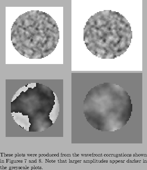
Figures 7 and
8 show the delay applied to the
wavefronts by the atmosphere after the tip-tilt
correction. Figure 7 shows the case
for
![]() wavelength and
Figure 8 the case for
wavelength and
Figure 8 the case for
![]() wavelength. Note that apart from the pixel
sampling in the images there is no obvious difference. This is because
the delay
wavelength. Note that apart from the pixel
sampling in the images there is no obvious difference. This is because
the delay ![]() from Equation 19 has only a
weak dependence on wavelength.
from Equation 19 has only a
weak dependence on wavelength.
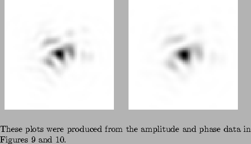
A larger difference appears when the atmospheric delays are converted
into optical amplitude and phase. The amplitude and phase in the pupil
plane are shown in Figures 9 and
10 for the same timestep as used for
Figures 7 and
8.
Figure 9 shows the amplitude and phase
at
![]() wavelength plotted as a function of position
in the AT aperture plane. The discontinuities in the phase occur when
the phase wraps around by
wavelength plotted as a function of position
in the AT aperture plane. The discontinuities in the phase occur when
the phase wraps around by ![]() radians. The same plots are shown in
Figure 10 for
radians. The same plots are shown in
Figure 10 for
![]() wavelength. It is clear that the phase perturbations are much more
severe at
wavelength. It is clear that the phase perturbations are much more
severe at
![]() due to the inverse relationship of the
phase
due to the inverse relationship of the
phase ![]() with wavelength seen in
Equation 19.
with wavelength seen in
Equation 19.
 |
 |
||
|
Figure 7
Atmospherically induced optical delay at one timepoint as a
function of position in one AT aperture plane at
|
Figure 8
Optical delay at
|
| In both plots the tip-tilt Zernike modes have been corrected across the telescope aperture, resulting in a discontinuity at the edge of the aperture. |
 |
 |
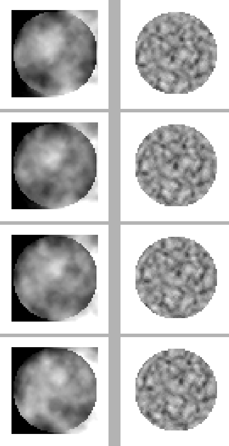
Example plots from ![]() later timesteps of the
simulations are shown in Figures 13 and
14.
later timesteps of the
simulations are shown in Figures 13 and
14.
Figure 13 shows the delay imposed on the
wavefronts by the simulated atmosphere as a function of position in
one of the AT aperture planes. The tip-tilt within the AT aperture has
been corrected by perfectly compensating the tip and tilt Zernike
modes, resulting in a discontinuity at the edges of the aperture in
this plot. The four images show four timesteps with the atmospheric
phase screens moving by ![]() in consecutive images in the
directions described in Section 3. Each atmospheric
layer has an equal effect on the wavefront phase.
in consecutive images in the
directions described in Section 3. Each atmospheric
layer has an equal effect on the wavefront phase.
Figure 14 shows the optical amplitude as a
function of position in the same AT aperture plane. It is clear that
the amplitude fluctuations are dominated by one of the layers moving
from the lower left to the upper right. The dominant layer is the
higher one (![]() above the telescope - see
Section 3.2).
above the telescope - see
Section 3.2).
 |
Robert Tubbs 平成16年11月18日