: Estimated performance of PRIMA : Detailed contributions : Detailed contributions 目次
In order to investigate potential sources of noise in the fringe tracking process, the simulations described in Section 3 were modified to include a simple fringe tracking algorithm. Optical propagation through the VLTI was not modelled - the spatially filtered output from two telescope simulations was simply combined to form an interferometer. In the fringe tracking algorithm, the phases of the seven spectral channels used in the simulation were adjusted so as to subtract the fringe offset measured in the previous timestep (or according to the piston mode if it was the first timestep). The seven channels were then combined to produce the two group delay tracking channels and the one phase tracking channel analogous to the PRIMA FSU spectral channels, as described in Section 3.2. The group delay tracking channels were then used to produce an estimate of the change in group delay, and this was used to find the nearest zero-point in the fringe phase.
One of the first interesting results to come out of these simulations
was just how difficult group delay estimation is using the two widely
spaced wavelength channels from the PRIMA FSU design, particularly
during periods of less-than-ideal seeing. When the stellar images at
the telescopes are distorted by wavefront corrugations across the
telescope apertures, the phases of the fringes in the group delay
tracking channels are also perturbed. This perturbation is different
in the two different spectral channels, which produces a substantial
error in the calculated group delay. This problem was partially solved
by low-pass filtering the group delay measurements, causing
perturbations due to the atmosphere to be averaged out over ![]() --
--![]() time units (where one time unit corresponds to the time taken for each
atmospheric layer to move
time units (where one time unit corresponds to the time taken for each
atmospheric layer to move ![]() , as discussed in
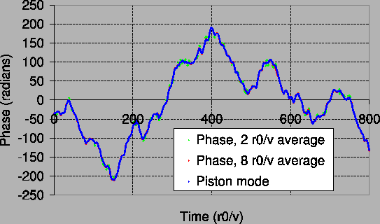
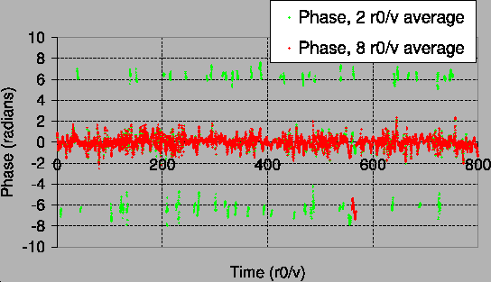
Section 3). The fringe tracking algorithm was then found
to perform very well, with fringe jumps detected only every few
hundred fringe coherence times. Example plots of the fringe tracking
performance are shown in Figures 21 and
22. If the group delay measurements are averaged
over too long a period, the algorithm is not able to track the motion
of the fringes due to the atmospheric piston mode fluctuations.
, as discussed in
Section 3). The fringe tracking algorithm was then found
to perform very well, with fringe jumps detected only every few
hundred fringe coherence times. Example plots of the fringe tracking
performance are shown in Figures 21 and
22. If the group delay measurements are averaged
over too long a period, the algorithm is not able to track the motion
of the fringes due to the atmospheric piston mode fluctuations.
 |
 |
These preliminary simulations have also been useful in determining
which factors will have the most impact on fringe tracking
performance, and hence which should be studied in more
detail. Simulations were performed with seeing of
![]() and seeing of
and seeing of
![]() at K band
(see Section 2.1 for an introduction to atmospheric
seeing - these numbers correspond approximately to the following two
sets of conditions: observing a target at low elevation under below
average seeing; and observing a target at the Zenith under excellent
seeing). Both the full aperture (
at K band
(see Section 2.1 for an introduction to atmospheric
seeing - these numbers correspond approximately to the following two
sets of conditions: observing a target at low elevation under below
average seeing; and observing a target at the Zenith under excellent
seeing). Both the full aperture (![]() ) and a stopped-down
aperture (
) and a stopped-down
aperture (![]() ) were simulated. A summary of the simulation
characteristics is presented in
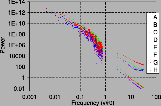
Table 4. Temporal power spectra of the fringe
motion are plotted in Figure 23 for these
simulations.
) were simulated. A summary of the simulation
characteristics is presented in
Table 4. Temporal power spectra of the fringe
motion are plotted in Figure 23 for these
simulations.
It is clear from the power spectra in Figure 23 that the fringe motion at high frequencies is dominated by the wavefront corrugations across the aperture in all the simulations, and the piston mode component (discussed in e.g. [9]) is negligible. Note that the piston mode component has a larger high frequency component with smaller aperture sizes as expected, but this is swamped by the effects of wavefront corrugations across the AT aperture, which are much smaller with the smaller aperture size. It is clear that the fringe tracking performance will be determined mostly by the effects of these wavefront corrugations, and that the slow drifts from the piston mode component will be much less important in optimising the fringe tracking algorithm.
 |
|
|||||||||||||||||||||||||
|
|
The maximum aperture diameter which can successfully used for fringe
tracking will be set by the amount of fringe jitter introduced by the
wavefront corrugations across the aperture. It is interesting to
compare the fringe jitter under different seeing conditions and with
different aperture diameters. In this case I have defined the jitter
as the residual fringe phase after the piston mode component has been
subtracted. There was no photon shot noise or detector noise in these
simulations, so this phase difference corresponded directly to the
effect of the wavefront corrugations across the aperture plane. A
summary of the simulation characteristics and results is presented in
Table 5 (the simulations are the same as those
presented in Table 4). The likelihood of fringe
jumps should be small as long as the RMS fringe jitter ![]() radian.
radian.
|
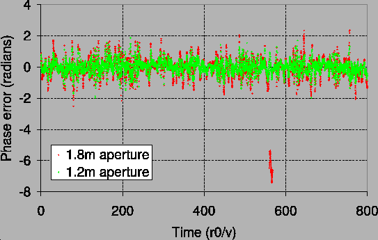
The phase jitter with the full diameter aperture under the poorer
seeing conditions (Simulation 1) is clearly much worse than the other
cases. Stopping down the AT aperture provides a very significant
reduction in the phase jitter, and appears a promising option at times
when fringe tracking becomes very unreliable. Note that the very high
phase jitter for Simulation 1 is partly due to a small number of very
large phase excursions including fringe jumps, an example of which is
shown in Figure 24. Note that the RMS phase
jitter is lower for the ![]() diameter aperture at all times,
however. The loss of stellar flux would make stopping down the
telescope aperture less appealing for faint stars.
diameter aperture at all times,
however. The loss of stellar flux would make stopping down the
telescope aperture less appealing for faint stars.
 |
Robert Tubbs 平成16年11月18日