Background

Producing an error budget for PRIMA astrometric observations will be a long and complicated process. In order to break up the work, the error calculation has been separated into a number of principle terms, with each term getting a section (or appendix) in this document. Each of these sections provides an introduction to the error term. A little more detail has been provided for some of the error terms, where that information was already available in existing documents. A substantial amount of further work will be required in order to complete the error budget.

One of the most difficult tasks has been to find the interdependencies of each of the different error terms. If one term in the error budget calculation is changed, this list of interdependencies can be used to work out which other components of the error budget calculation will be effected by the change. Tables of interdependencies can be seen in Appendix O. These include both direct dependencies (the terms in the error budget which are directly effected by a change) and indirect dependencies (those terms which are effected indirectly through a change in an intermediate term in the calculations).

In order to introduce the terminology used in this report I will first give an introduction to atmospheric turbulence and interferometry. In the standard classical theory, light is treated as an oscillation in a field $\psi$. For monochromatic plane waves arriving from a distant point source with wave-vector $\mathbf{k}$:

$$\psi_{u} \left(\mathbf{r},t\right) = A_{u}e^{i\left (\phi_{u} + 2\pi\nu t + \mathbf{k}\cdot\mathbf{r} \right )}$$ (1)

where $\psi_{u}$ is the complex field at position $\mathbf{r}$ and time $t$, with real and imaginary parts corresponding to the electric and magnetic field components, $\phi_{u}$ represents a phase offset, $\nu$ is the frequency of the light determined by $\nu=c\left \vert \mathbf{k} \right \vert / \left ( 2 \pi \right )$, and $A_{u}$ is the amplitude of the light.

The photon flux in this case is proportional to the square of the amplitude $A_{u}$, and the optical phase corresponds to the argument of the complex variable $\psi_{u}$. As wavefronts pass through the Earth's atmosphere they may be perturbed by refractive index variations in the atmosphere. Figure 1 shows schematically a turbulent layer in the Earth's atmosphere perturbing planar wavefronts before they enter a telescope. The perturbed wavefront $\psi_{p}$ may be related at any given instant to the original planar wavefront $\psi_{u} \left(\mathbf{r},t\right)$ in the following way:

$$\psi_{p} \left(\mathbf{r},t\right) = \left ( \chi_{p} \left(... ...mathbf{r},t\right)}\right ) \psi_{u} \left(\mathbf{r},t\right)$$ (2)

where $\chi_{p} \left(\mathbf{r},t\right)$ represents the fractional change in wavefront amplitude and $\phi_{p} \left(\mathbf{r},t\right)$ is the change in wavefront phase introduced by the atmosphere. From here on in this document, $\phi_{p} \left(\mathbf{r},t\right)$ will be called the optical phase (although strictly it is the perturbation in the optical phase in comparison to an unperturbed light beam). Similarly, in discussions of atmospheric effects $\chi_{p} \left(\mathbf{r},t\right)$ will be called the wavefront amplitude although it is actually a normalised form of the amplitude.

図 1: Schematic diagram illustrating how optical wavefronts from a distant star may be perturbed by a turbulent layer in the atmosphere. The vertical scale of the wavefronts plotted is highly exaggerated.

A description of the nature of the wavefront perturbations introduced by the atmosphere is provided by the Kolmogorov model developed by Tatarksi ([1]) and Kolmogorov ([2,3]). This model is supported by a variety of experimental measurements and is widely used in simulations of astronomical instruments. The model assumes that the wavefront perturbations are brought about by variations in the refractive index of the air. These refractive index variations lead directly to phase fluctuations described by $\phi_{p} \left(\mathbf{r},t\right)$, but any amplitude fluctuations are only brought about as a second-order effect while the perturbed wavefronts propagate from the perturbing atmospheric layer to the telescope. The performance of interferometers is dominated by the phase fluctuations $\phi_{p} \left(\mathbf{r},t\right)$, although the amplitude fluctuations described by $\chi_{p} \left(\mathbf{r},t\right)$ introduce intensity variations (scintillation) in the interferometric signal.

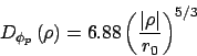
The spatial phase fluctuations at an instant in time in a Kolmogorov model are usually assumed to have a Gaussian random distribution with the following second order structure function:

$$D_{\phi_{p}}\left(\mathbf{\rho} \right) = \left \langle \lef... ...{\rho} \right ) \right \vert ^{2} \right \rangle _{\mathbf{r}}$$ (3)

where $D_{\phi_{p}} \left ({\mathbf{\rho}} \right )$ is the atmospherically induced variance between the phase at two parts of the wavefront separated by a distance $\mathbf{\rho}$ in the aperture plane, and $\left < \ldots \right >$ represents the ensemble average.

The structure function of [1] can be described in terms of a single parameter $r_{0}$:

$$D_{\phi_{p}} \left ({\mathbf{\rho}} \right ) = 6.88 \left ( ... ...\left \vert \mathbf{\rho} \right \vert}{r_{0}} \right ) ^{5/3}$$ (4)

$r_{0}$ indicates the ``strength'' of the phase fluctuations as it corresponds to the diameter of a circular telescope aperture at which atmospheric phase perturbations begin to seriously limit the image resolution. Typical $r_{0}$ values for K band ( $2.2\mbox{ $\mu m$}$ wavelength) observations at good sites are $40$--$90$ $cm$. Fried ([4]) noted that $r_{0}$ also corresponds to the aperture diameter $d$ for which the variance $\sigma ^{2}$ of the wavefront phase averaged over the aperture comes approximately to unity:

$$\sigma ^{2}=1.0299 \left ( \frac{d}{r_{0}} \right )^{5/3}$$ (5)

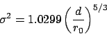
Equation 5 represents a commonly used definition for the atmospheric coherence length $r_{0}$.