After becoming familiar with the data structure, the I/O routines, the basic tools, the photometry, the spectroscopy, and the concept of MIA, we will continue with the analysis of the interferometric data of the calibrator HD 10380.

Getting started

As a first step start "Gorgonzola" by typing

  calfile=midigui(dir='<path>')

where <path> is the directory where the interferometric and photometric data are stored. Now select the data set for the fringe trackimg (OBS_FRINGE_TRACK_FOURIER) and the two photometric measurements (OBS_PHOTOMETRY_CHOP) by marking the first column and pressing the button "SELECT". Then the names of the files are stored for this example in the array calfile. It is important that the data set containing the fringes is stored as the first entry in this array. If the photometric observations have been performed before the fringe-tracking was done, please rearrange the array by typing

  calfile=SHIFT(calfile,1)

(The example data of HD 10380 was taken in the usual order, so you don't have to do this).

Now the main routine of the MIA software package xmdv can be started with

  cal=xmdv(calfile)

There are sevaral options you can give after calfile:

MASKFILE=filename	uses the specified file as mask to extract the photometric flux and the fringe signal. This can be the mask of photometry A or B or any other mask you found somewhere.
MASKWIDTH=w	create a mask that is wider by a factor w than the default. This works with the mask created by averaging mask A and B, and with the mask created from fringedata, but not with a mask given via the MASKFILE keyword!
NOISEFILE=filename	specifies a file to be prepended to the fringe track data. The idea is to use a fringe search file, which (hopefully) contains scans without any fringes (even at long wavelengths).
/DISPERSEDTRACK or DISPERSEDTRACK=bins	Simple support for dispersed fringe tracking. The fringe amplitude is not computed in white light, but in a number of wavelength-bins given by bins (default: 20). This should be the default, but it hasn't been fully tested yet.
/SHOW_TRACES	create two Postscript files showing the traces of the photometric masks and of the mask that is used for extracting the data.

The Masks

First, for both AOPEN and BOPEN the mask for each of the two windows (I1&I2) is created with the chop_nod_disp routine. After calculating the mean, i.e.

  Mean [ Mask(AOPEN,I1), Mask(BOPEN,I1) ] = Mask(NEW,I1)
  Mean [ Mask(AOPEN,I2), Mask(BOPEN,I2) ] = Mask(NEW,I2)

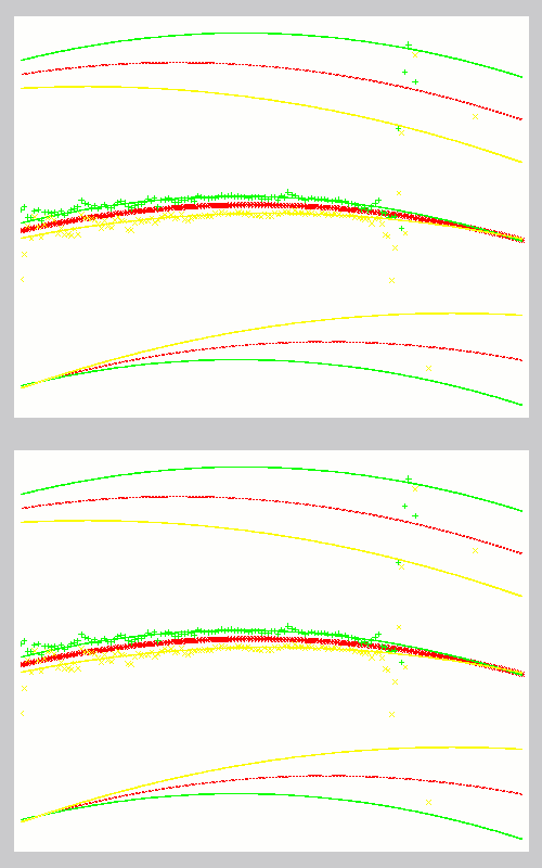
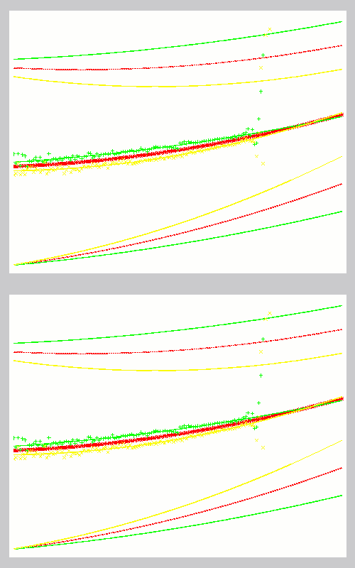
the NEW masks can be used to extract the fringes and the photometry. The postscript files '<path>/traces_win1.ps' (I1) and '<path>/traces_win2.ps' (I2) shown below visualize this averaging process. To access the parameters of the input masks (AOPEN, BOPEN) you can use the command

  tr = cal->get_trace(i)

after the next steps will have been finished. The index iselects the dataset: 0 = AOPEN or 1 = BOPEN. If the option /WIN2 is set, the trace of window 2 will be returned, else that of window 1. The available parameters of the traces are

• tr.trace - measured position of the peak as function of pixel number
• tr.FWHM - the measured FWHM
• tr.fluxmax - height of the peak
• tr.range - indices of good trace measurements
• tr.nRange - the number of good measurements
• trace_coeff - coefficients of the trace-polynomial
• sigma_coeff - coefficients of the sigma-polynomial

To load or create other masks please use the options described above.

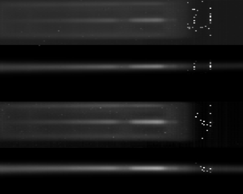
Now OirGetMeanRMS is used to calculate the root mean square of the fringe-tracking data. After weighting the resulting images with the averaged masks from the photometric datasets (see above) the user can decide whether the masks are well fitting for the fringe-tracking data too.

If the user confirms that the masks are satisfying, the routine starts to calculate all the required informations. Unfortunately, there is not much we can do if the masks are not satisfying. The only way to influence the mask is to provide another mask-file.