Included Runs
L025N0188_Thermal_non_equilibrium
Basic
- Box-size: \(25\; \rm{Mpc}\)
- Dark matter particle mass: \(1.94 \times 10^{7}\; \rm{M}_\odot\)
- Gas particle mass: \(1.47 \times 10^{7}\; \rm{M}_\odot\)
- Snapshot \(z=2.00\), \(a=0.33\)
Particle Numbers
Cube root of Dark Matter particle number: 298
| Gas | Dark Matter | Star | Black Hole |
|---|---|---|---|
| 6495799 | 26578688 | 148338 | 540 |
Gravitational Softening
| Baryons | Dark Matter | ||
|---|---|---|---|
| Max Physical | Comoving | Max Physical | Comoving |
| \(1.4\; \rm{kpc}\) | \(3.6\; \rm{kpc}\) | \(1.4\; \rm{kpc}\) | \(3.6\; \rm{kpc}\) |
Stars
| Parameter | Value |
|---|---|
| Max time-step of young stars | \(1\; \rm{Myr}\) |
| Transition from young to old | \(3.4 \times 10^{38}\; \rm{Myr}\) |
| Max time-step of old stars | \(3.4 \times 10^{38}\; \rm{Myr}\) |
| Transition from old to unlimited | \(40\; \rm{Myr}\) |
Star Formation
| Parameter | Value |
|---|---|
| Star Formation Model | SchmidtLaw |
| Temperature Ceiling | \(0\; \rm{K}\) |
| Virial Parameter | \(1\) |
| Star-formation efficiency (Schmidt law) | \(0.01\) |
| Threshold SF \(n_{\rm H, max}\) | \(3.4 \times 10^{38}\) cm\(^{-3}\) |
| Immediate SF \(n_{\rm H, max}\) | \(3.4 \times 10^{38}\) cm\(^{-3}\) |
Stellar Feedback
| Parameter | Value |
|---|---|
| SNII Energy | \(1 \times 10^{51}\; \rm{erg}\) |
| SNIa Energy | \(1 \times 10^{51}\; \rm{erg}\) |
| \(f_{\rm E, min}\) | \(0.1\) |
| \(f_{\rm E, max}\) | \(4\) |
| \(\sigma_{\rm P}\) | \(0.3\) |
| \(P_{\rm E,pivot} / k_{\rm B}\) | \(8 \times 10^{3}\) K cm\(^{-3}\) |
| \(n_{\rm Z}\) | \(0\) |
| \(Z_{\rm E,pivot}\) | \(0.0134\) |
| \(n_{\rm n}\) | \(0\) |
| \(n_{\rm E,pivot}\) | \(0.67\) cm\(^{-3}\) |
| \(f_{\rm kinetic}\) | \(0.1\) |
| SNII \(v_{\rm kick}\) | \(50\; \rm{km} / \rm{s}\) |
| SNII var-dT pivot temperature \(\Delta T_{\rm pivot}\) | \(3.16 \times 10^{6}\; \rm{K}\) |
| SNIa var-dT pivot temperature \(\Delta T_{\rm pivot}\) | \(3.16 \times 10^{6}\; \rm{K}\) |
| SNII var-dT pivot density \(n_{\rm H, pivot}\) | \(0.6\) cm\(^{-3}\) |
| SNIa var-dT pivot density \(n_{\rm H, pivot}\) | \(0.6\) cm\(^{-3}\) |
| SNII var-dT min temperature \(\Delta T_{\rm min}\) | \(3.16 \times 10^{6}\; \rm{K}\) |
| SNIa var-dT min temperature \(\Delta T_{\rm min}\) | \(3.16 \times 10^{6}\; \rm{K}\) |
| SNII var-dT max temperature \(\Delta T_{\rm max}\) | \(3.16 \times 10^{7}\; \rm{K}\) |
| SNIa var-dT max temperature \(\Delta T_{\rm max}\) | \(3.16 \times 10^{7}\; \rm{K}\) |
| SNII var-dT slope | \(0.667\) |
| SNIa var-dT slope | \(0.667\) |
| Use Stellar Winds | \(1\) |
| Use Radiation Pressure | \(1\) |
| Early Feedback \(v_{\rm kick}\) | \(50\; \rm{km} / \rm{s}\) |
| Use HII Regions | \(1\) |
| SNII yield factor H | \(1\) |
| SNII yield factor He | \(1\) |
| SNII yield factor C | \(1.5\) |
| SNII yield factor N | \(1\) |
| SNII yield factor O | \(1\) |
| SNII yield factor Ne | \(1\) |
| SNII yield factor Mg | \(1.5\) |
| SNII yield factor Si | \(1\) |
| SNII yield factor Fe | \(1\) |
Gas Cooling
CHIMES
cooling_rates
| Parameter | Value |
|---|---|
| Maximum Value of Gas-Dust Boost | \(1\) |
| Min Density in Gas-Dust Boost \(n_{\rm min}\) | \(0.1\) cm\(^{-3}\) |
| Max Density in Gas-Dust Boost \(n_{\rm max}\) | \(100\) cm\(^{-3}\) |
Dust
| Parameter | Value |
|---|---|
| Dust Model | Trayford et. al (2024) |
| With Coupling to Cooling | \(1\) |
| Clumping Factor Mode | variable |
| Clumping Factor | \(100\) |
| Min Density in Clumping Factor \(n_{\rm min}\) | \(0.1\) cm\(^{-3}\) |
| Max Density in Clumping Factor \(n_{\rm max}\) | \(100\) cm\(^{-3}\) |
Entropy Floor
No entropy floor present
Chemistry
| Parameter | Value |
|---|---|
| Metal diffusion constant | \(0.01\) |
AGN feedback
Parameters of the variable AGN \(\Delta T\) model
| \(\Delta T_{\rm min}\) | \(\Delta T_{\rm max}\) | \(\Delta T_{\rm pivot}\) | \(M_{\rm BH,pivot}\) | \(\rm Slope\) |
|---|---|---|---|---|
| \(3.16 \times 10^{6}\; \rm{K}\) | \(3.16 \times 10^{9}\; \rm{K}\) | \(3.16 \times 10^{9}\; \rm{K}\) | \(3.16 \times 10^{8}\; \rm{M}_\odot\) | 1.0 |
Other AGN parameters
| Parameter | Value |
|---|---|
| AGN Feedback Model | MinimumDistance |
| Use Deterministic Feedback | \(1\) |
| Coupling efficiency | \(0.1\) |
| Radiative efficiency | \(0.1\) |
| BH Subgrid Seed Mass | \(3.16 \times 10^{5}\; \rm{M}_\odot\) |
| Seed Halo Mass | \(5 \times 10^{10}\; \rm{M}_\odot\) |
| Target number of particles to heat N\(_{\rm heat}\) | \(1\) |
| Use sub-grid gas properties | \(1\) |
| Use Multi-phase Bondi | \(0\) |
| Use Krumholtz Accretion | \(1\) |
| Use Krumholtz Vorticity | \(1\) |
| Use Angular Momentum Limiter | \(0\) |
| Viscous \(\alpha\) | |
| Use Nibbling | \(1\) |
| Minimal Gas Mass For Nibbling | \(6.4 \times 10^{6}\; \rm{M}_\odot\) |
| Minimum BH time-step | \(100\; \rm{yr}\) |
| Maximal Reposition Mass | |
| Use Reposition Velocity Threshold | \(0\) |
| Maximal Reposition Velocity Offset | \(c_{s, {\rm BH}}\) |
| Minimal Reposition Velocity Threshold | |
| Set Black Hole Reposition Speed | \(0\) |
| Repositioning Speed Normalisation | |
| Black Hole Merger Threshold Type | DynamicalEscapeVelocity |
| Black Hole Merger Max Distance Ratio | \(3\) |
| Use Black Hole Accretion Boost Factor | \(0\) |
| Boost \(\alpha\) | |
| Boost \(\beta\) | |
| Boost \(n_{\rm norm}\) | cm\(^{-3}\) |
Code Setup
- Code info: SWIFT (hawk-scaling-test) v0.9.0-2707-g80d9af7b-dirty 2024-08-15 17:39:21 +0200
- Compiler info: LLVM/Clang (19.0.0) Open MPI v5.0.3 (MPI std v3.1)
- Hydrodynamics: SPHENIX (Borrow+ 2020) Quartic spline (M5) in 3D $\eta$ = 1.23 (64.90 $N_{ngb}$) $C_{\rm CFL}$ = 0.20
Ages
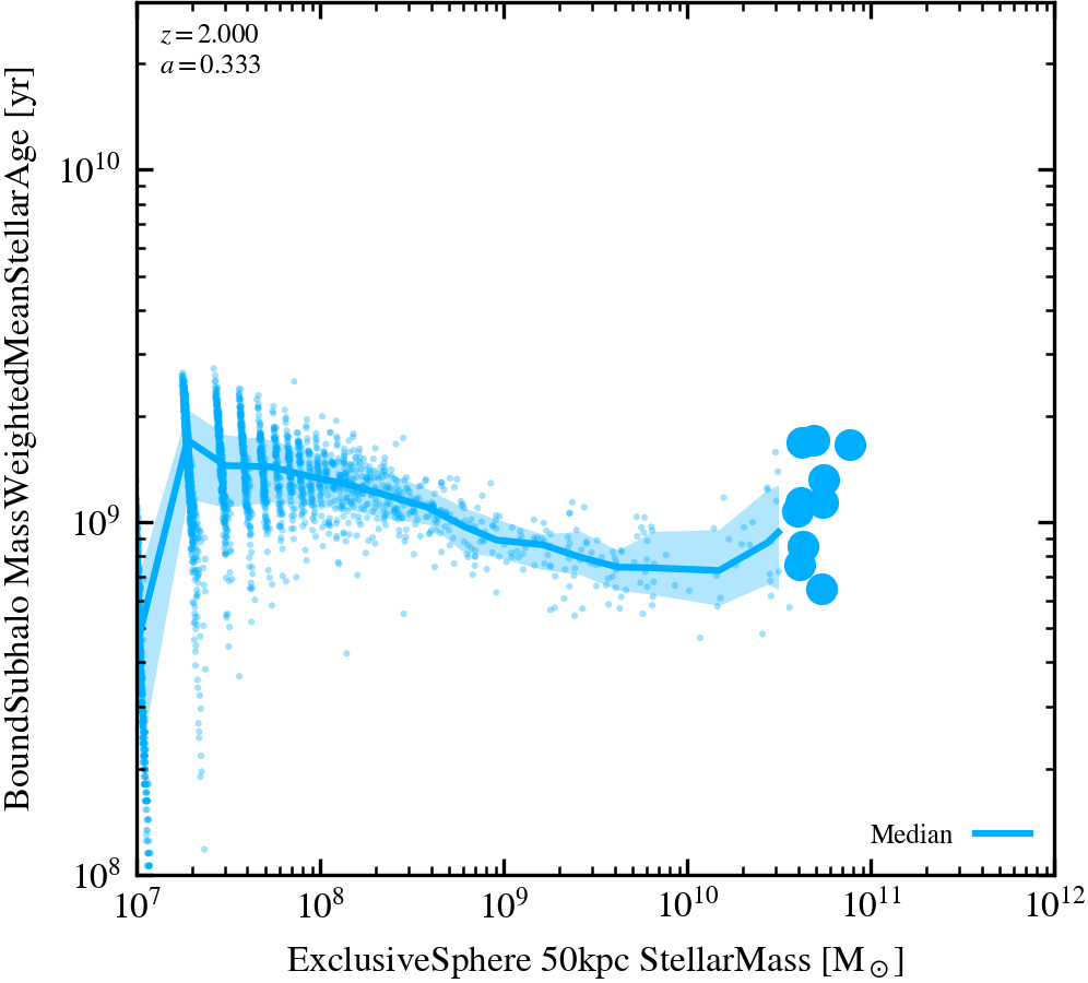
Stellar mass - Stellar age relation (50 kpc aperture)
Median age of stars within the 50 kpc 3D aperture of each galaxy.
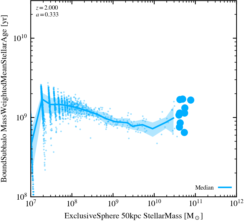
Stellar mass - Stellar age relation (50 kpc aperture, centrals only)
Median age of stars within the 50 kpc 3D aperture of each galaxy, showing central galaxies only.
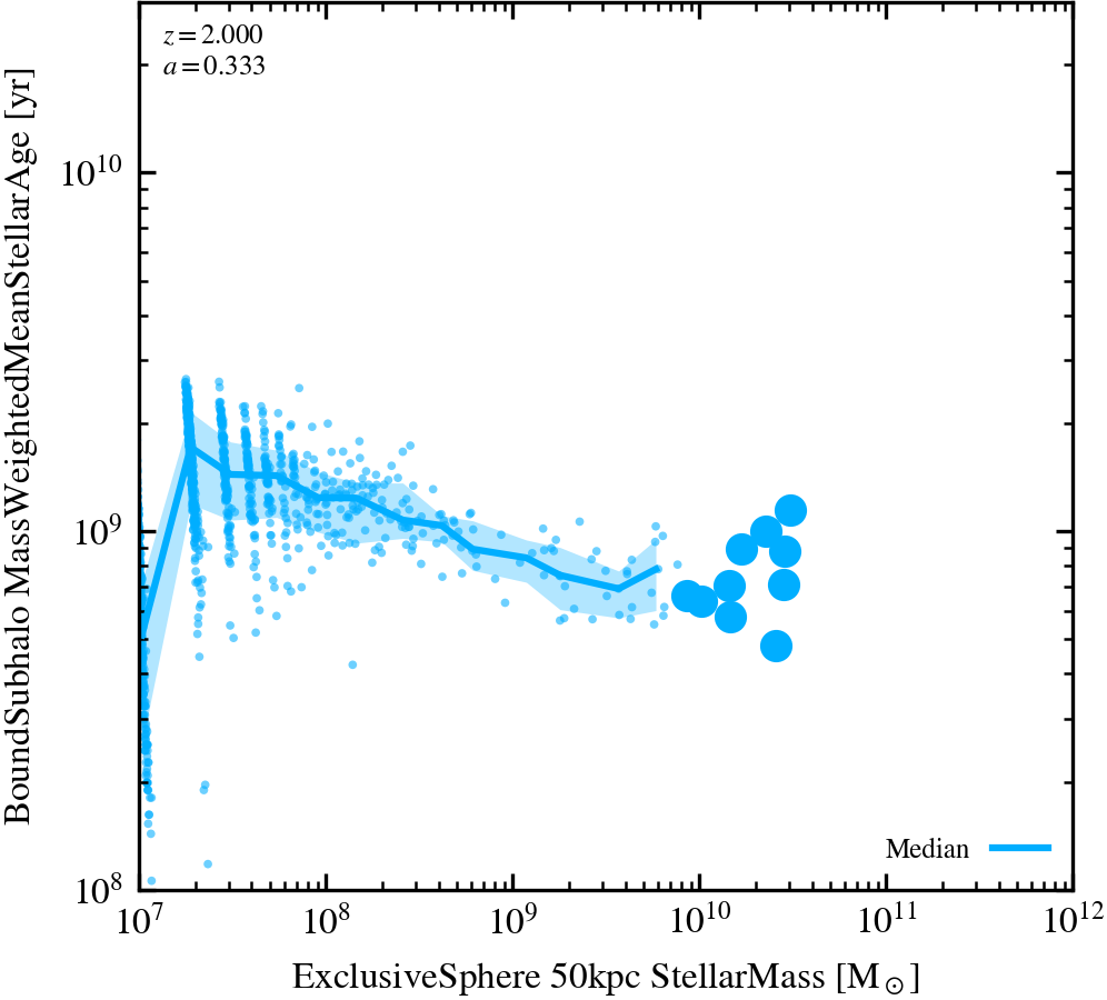
Stellar mass - Stellar age relation (50 kpc aperture, satellites only)
Median age of stars within the 50 kpc 3D aperture of each galaxy, showing satellite galaxies only.
Baryon Fractions
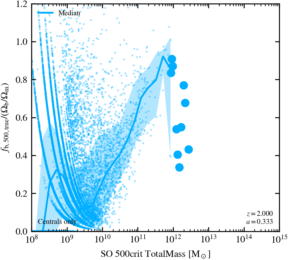
Halo baryon fractions within $R_{500}$
Baryon (gas + stars) fractions within $R_{500}$ normalised by the cosmic mean. These are 'true' values, i.e. no cut or observational correction was applied.
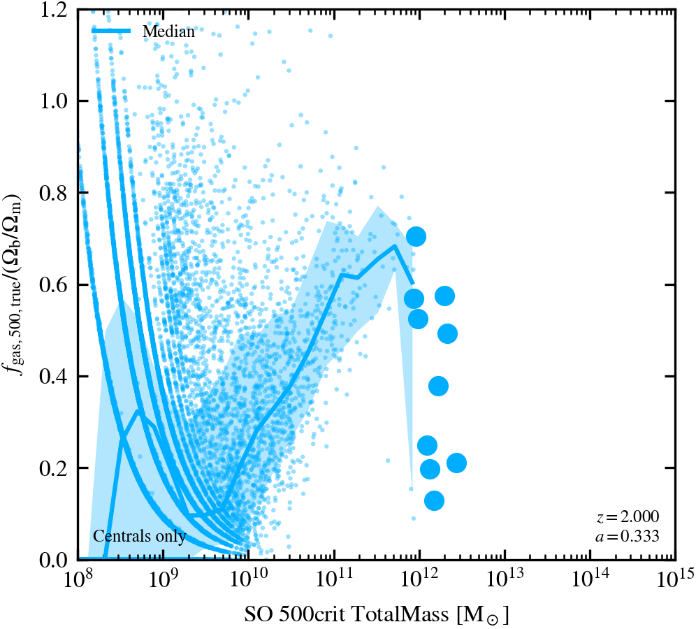
Halo gas fractions within $R_{500}$ (no hydrostatic bias)
Gas fractions within $R_{500}$ normalised by the cosmic mean. These are 'true' values, i.e. no cut or observational correction was applied. The observational data does not include any correction for hydrostatic bias.
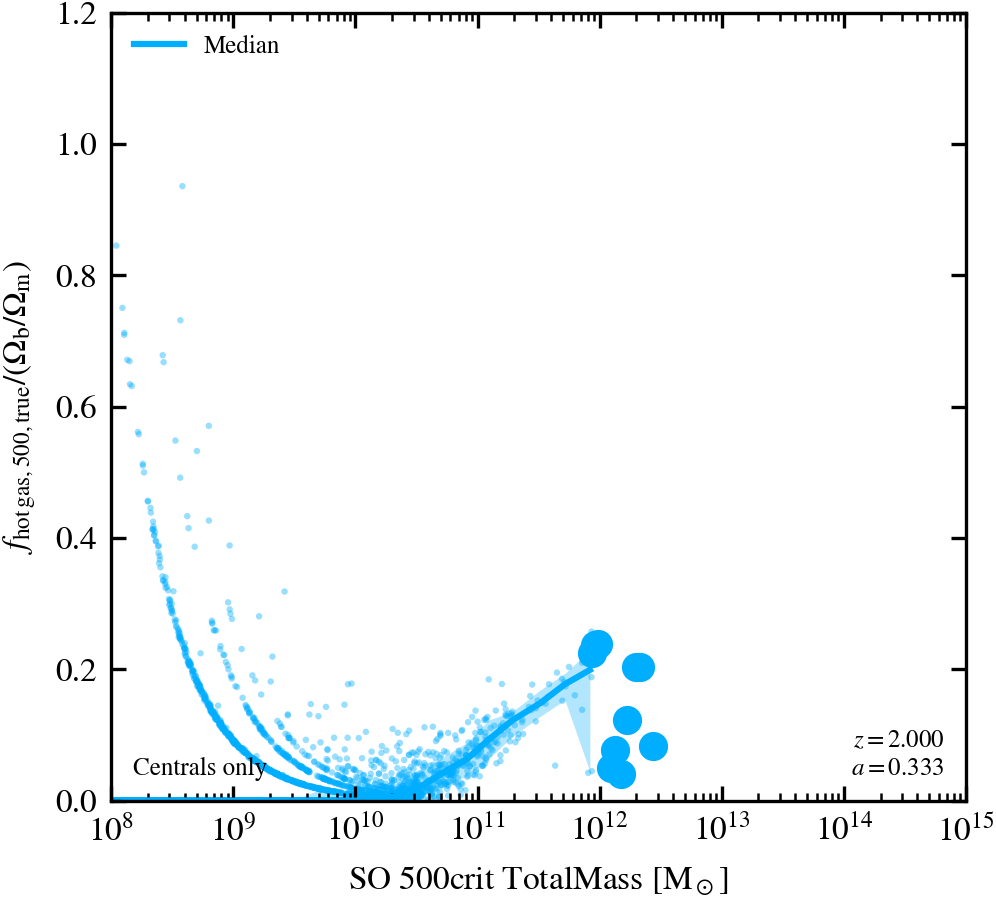
Halo hot gas fractions within $R_{500}$ (no hydrostatic bias)
Fraction of halo mass within $R_{500}$ in hot ($T>10^5$K) gas, normalised by the cosmic mean. These are 'true' values, i.e. no cut or observational correction was applied. The observational data does not include any correction for hydrostatic bias.
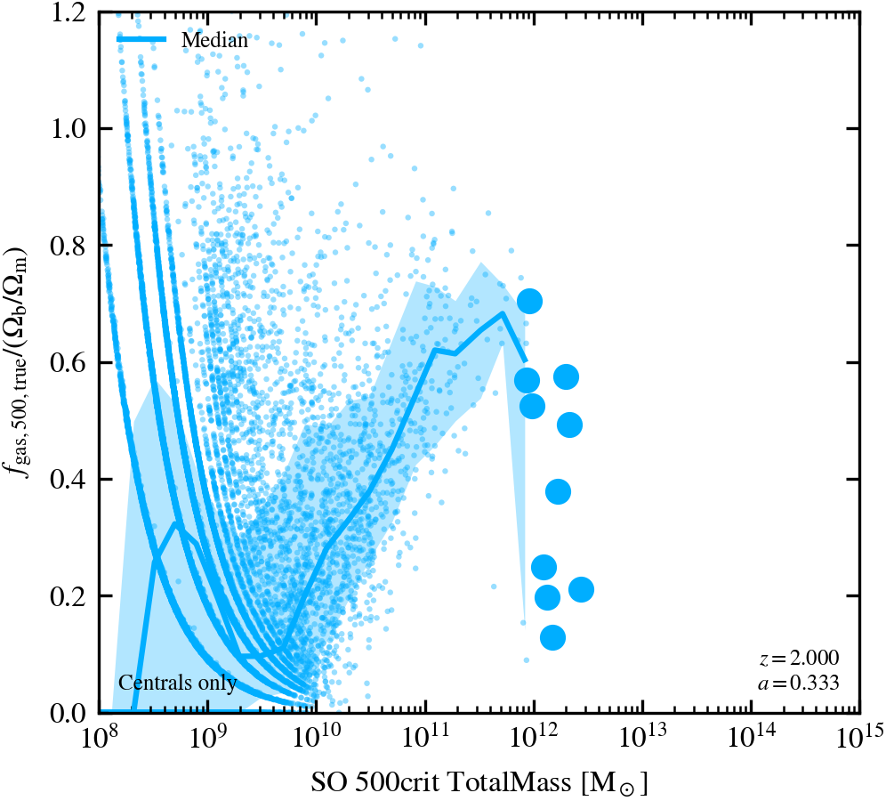
Halo gas fractions within $R_{500}$ (with hydrostatic bias)
Gas fractions within $R_{500}$ normalised by the cosmic mean. These are 'true' values, i.e. no cut or observational correction was applied. The observational data was compiled from 10+ HSE data sets (Kugel et al., in prep.), and includes the -0.75 dex hydrostatic bias correction factor used for FLAMINGO.
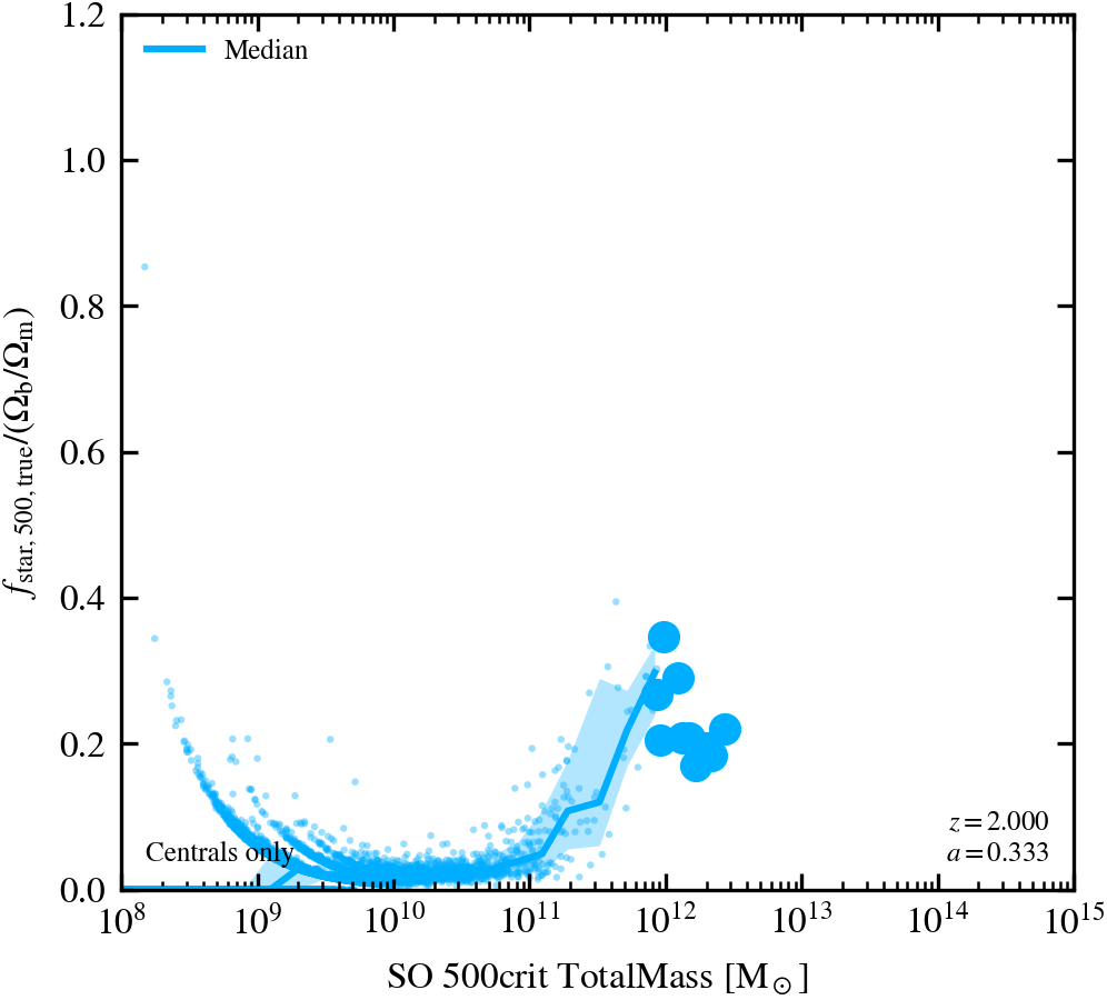
Halo stellar fractions within $R_{500}$
Stellar fractions within $R_{500}$ normalised by the cosmic mean. These are 'true' values, i.e. no cut or observational correction was applied.
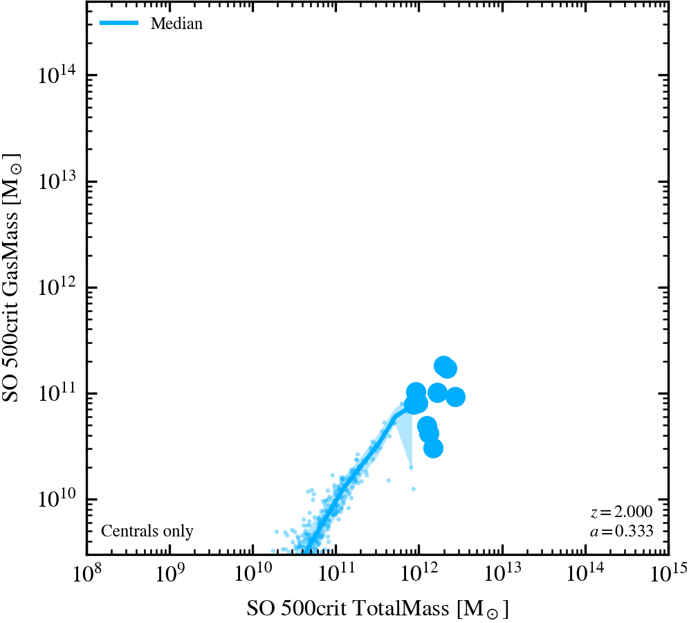
Halo gas masses within $R_{500}$
Gas masses within $R_{500}$. These are 'true' values, i.e. no cut or observational correction was applied.
Black Holes
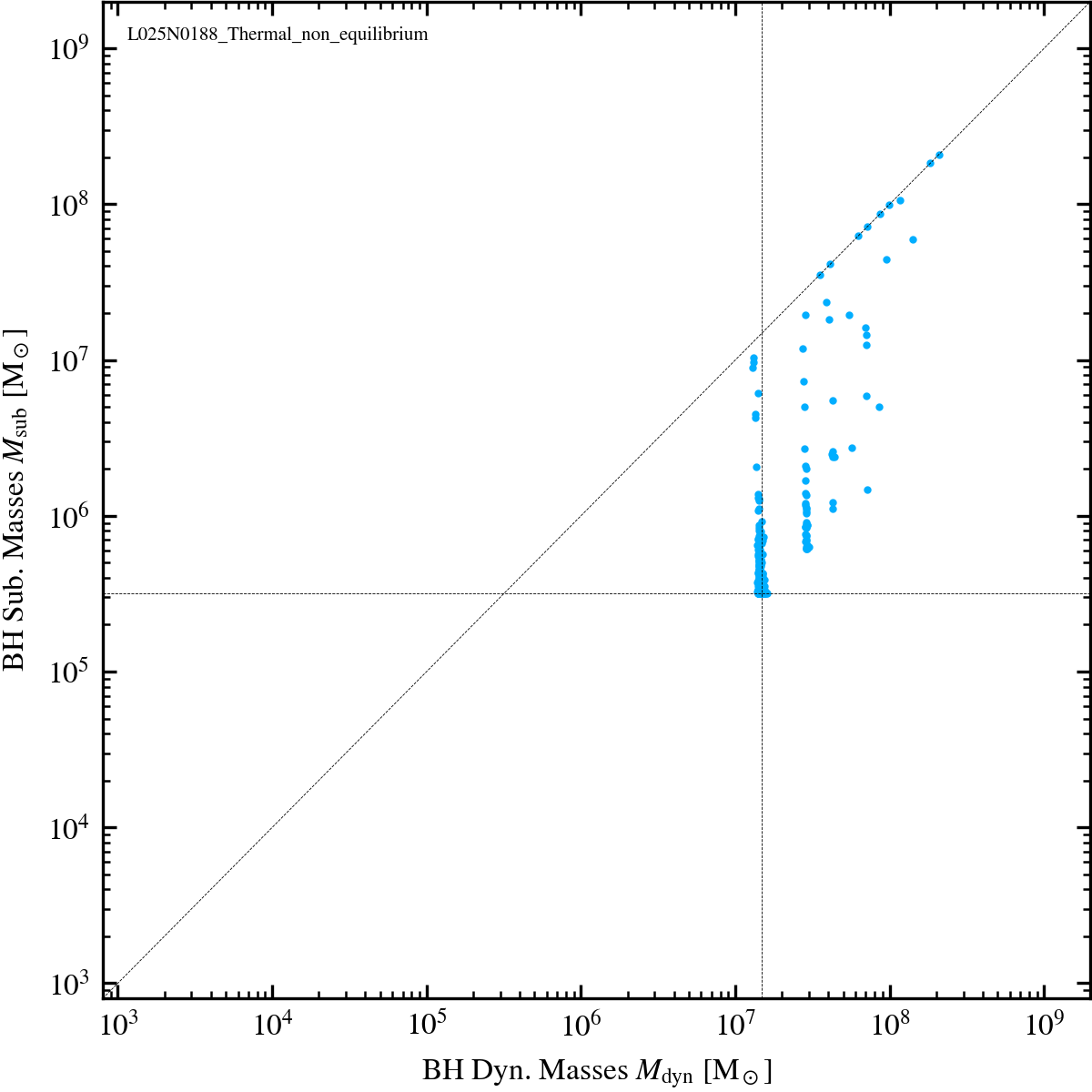
Black Hole Dynanmical and Subgrid Masses
Relation between black hole particle (dynamical) masses and subgrid masses. The vertical dashed lines shows the primordial gas particle mass and the horizontal dashed lines corresponds to the black hole seed mass.
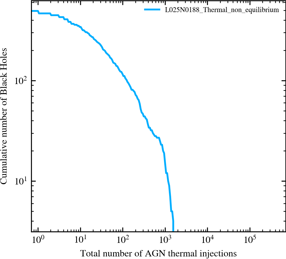
Cumulative number of AGN thermal injections
The cumulative number of black holes (summed from right to left) with a given total number of thermal energy injections (less than or equal to the number of particles heated) the black hole has had throughout the simulation.
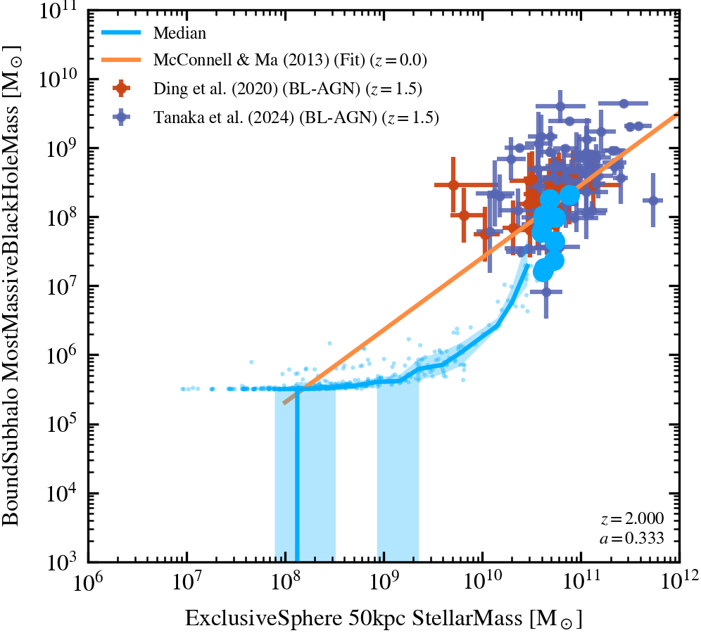
Stellar Mass-Black Hole Mass relation (50 kpc Stellar Mass)
SMBHM relation. Note that the stellar velocity dispersion is measured in observations in a fixed 1 kpc aperture
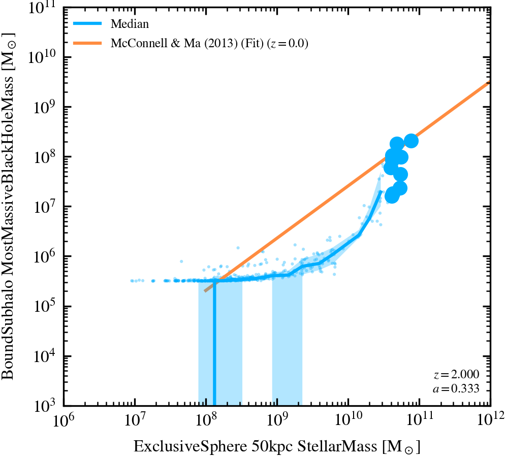
Stellar Mass-Black Hole Mass relation (50 kpc Stellar Mass)
SMBHM relation. The binned observational data are obtained by combining BH mass measurements for galaxies of different morphologies (Graham 2023) and passive vs. active galaxies (Terrazas et al. 2017) with dependencies on stellar mass of morphological types (Moffett et al. 2016, from the GAMA survey) and quenched fractions (Gilbank et al. 2010, SDSS).
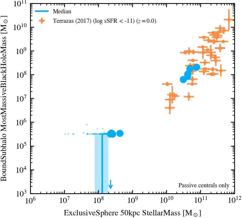
Stellar Mass-Black Hole Mass relation (50 kpc Stellar Mass) for passive central galaxies.
Stellar Mass-Black Hole Mass relation using a 30 kpc stellar mass aperture. Only passive (z=0 sSFR threshold is 0.01 / Gyr, z>0 is 0.2/t_H(z)) central galaxies are included.
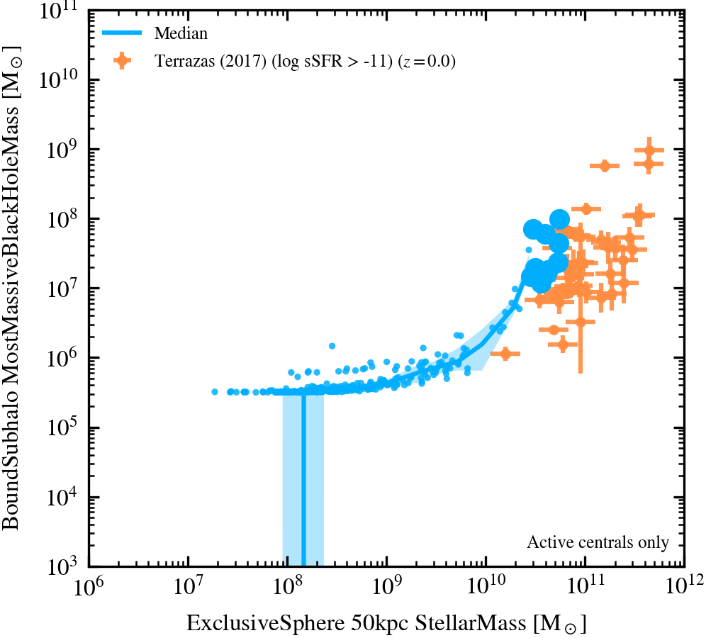
Stellar Mass-Black Hole Mass relation (50 kpc Stellar Mass) for active central galaxies.
Stellar Mass-Black Hole Mass relation using a 50 kpc stellar mass aperture. Only active (z=0 sSFR threshold is 0.01 / Gyr, z>0 is 0.2/t_H(z)) central galaxies are included.
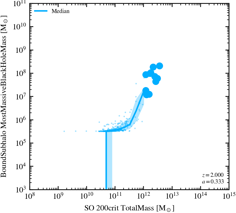
Halo Mass-Black Hole Mass relation
Presented for comparison between schemes as halo mass varies significantly less between models and runs.
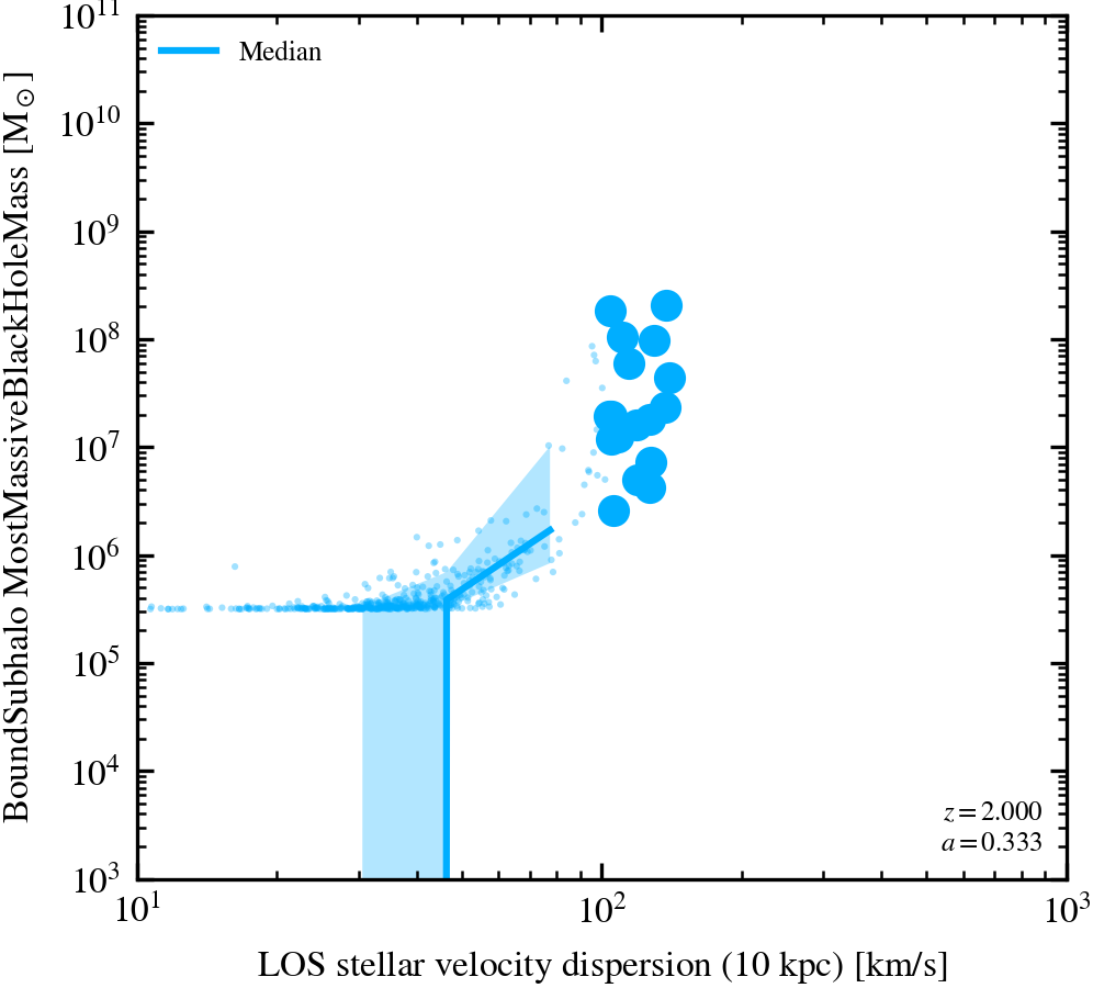
LOS Stellar Velocity Dispersion-Black Hole Mass relation (10 kpc)
The 3D stellar velocity dispersion is converted into a LOS velocity dispersion using a $1/\sqrt{3}$ correction factor. The stellar velocity dispersion from Sahu et al. (2016) was measured using a fixed 1 kpc aperture, while that from Saglia et al. (2016) was measured using the half-light radius aperture.
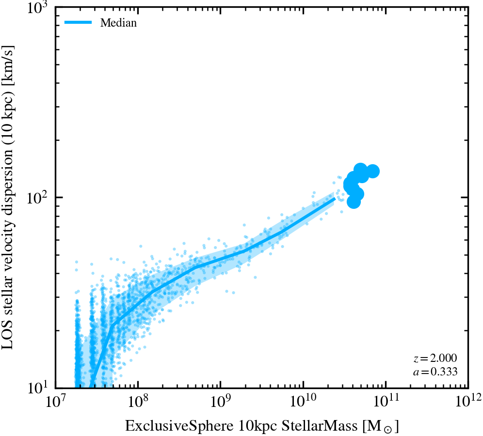
Stellar Mass-LOS Stellar Velocity Dispersion relation (10 kpc)
The 3D stellar velocity dispersion is converted into a LOS velocity dispersion using a $1/\sqrt{3}$ correction factor.
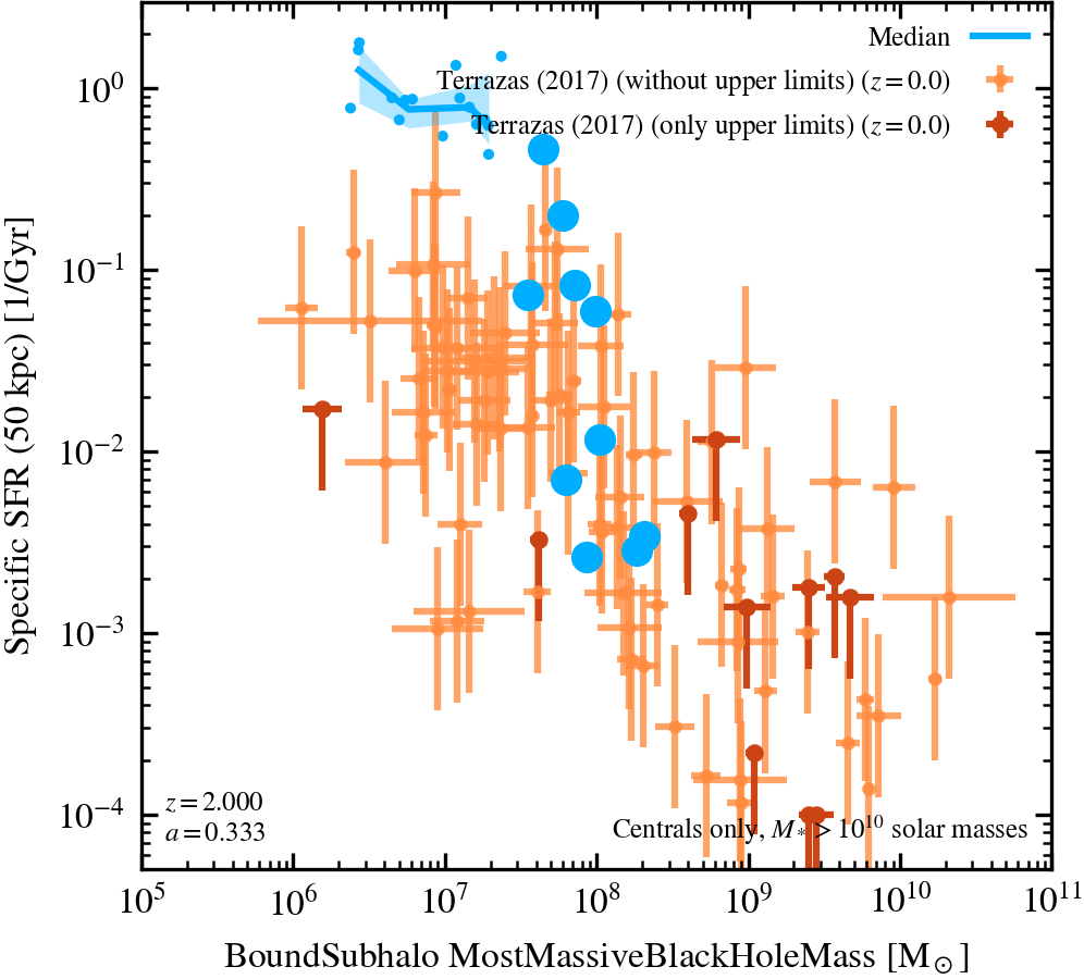
Black Hole Mass - sSFR relation (50 kpc sSFR)
Black Hole Mass - sSFR mass relation for galaxies with stellar mass $>10^{10}$ solar masses.
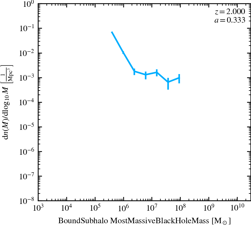
Black Hole Mass Function
The mass function of black holes (active and non-active).
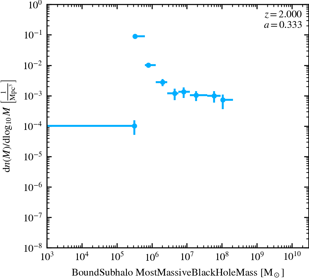
Black Hole Mass Function (adaptive)
The mass function of black holes (active and non-active), using adaptive binning.
Black Holes - Growth
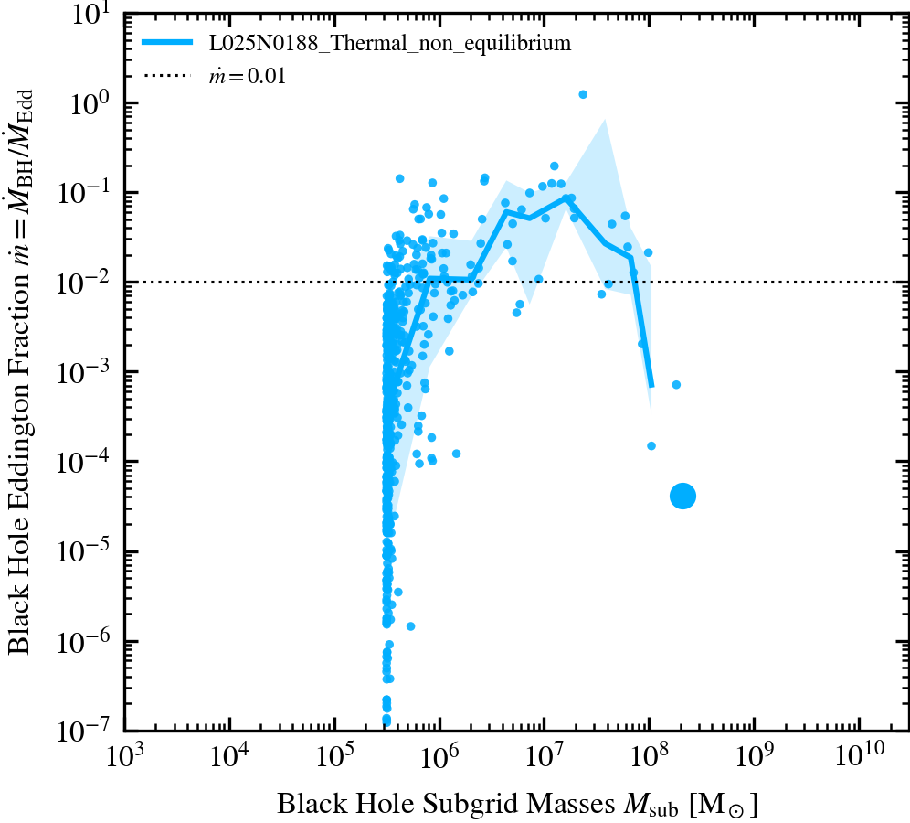
Black Hole Eddington Fraction - Mass Relation
The relation between black hole Eddington fraction and subgrid mass.
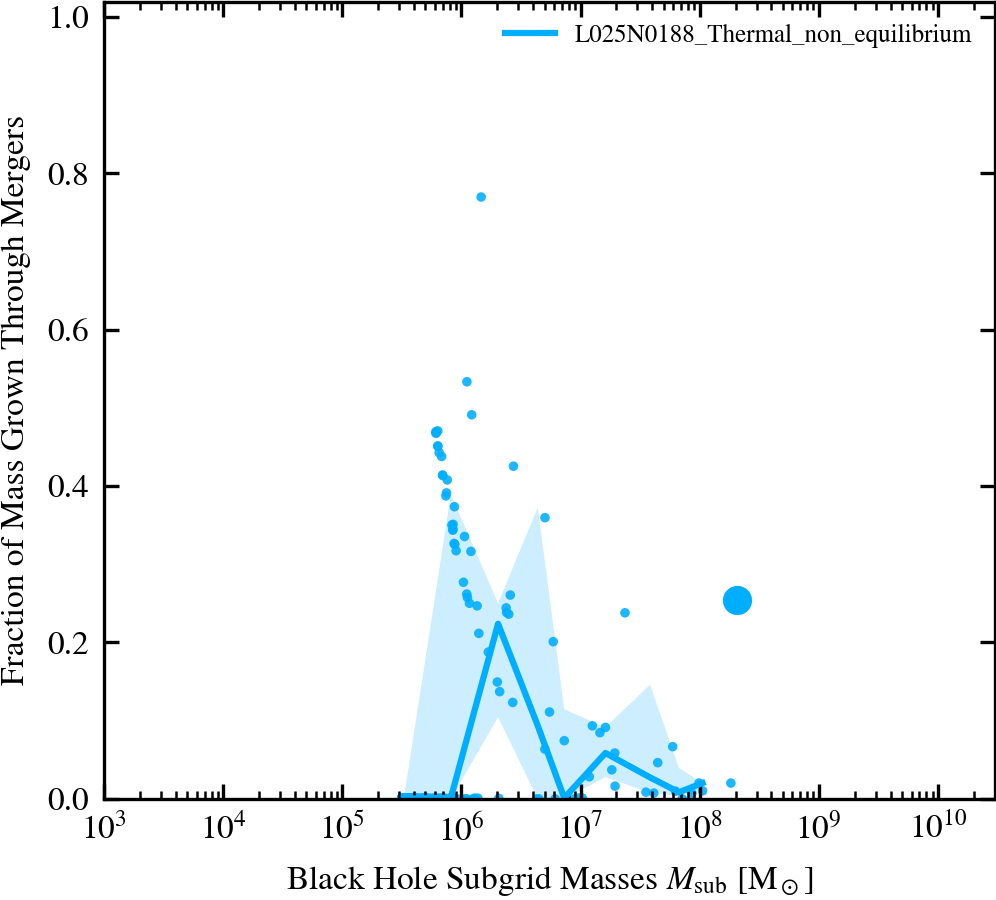
Black Hole Merger Mass Fractions - Mass Relation
The fraction of subgrid mass growth through mergers versus subgrid mass.
Black Holes - Radiation
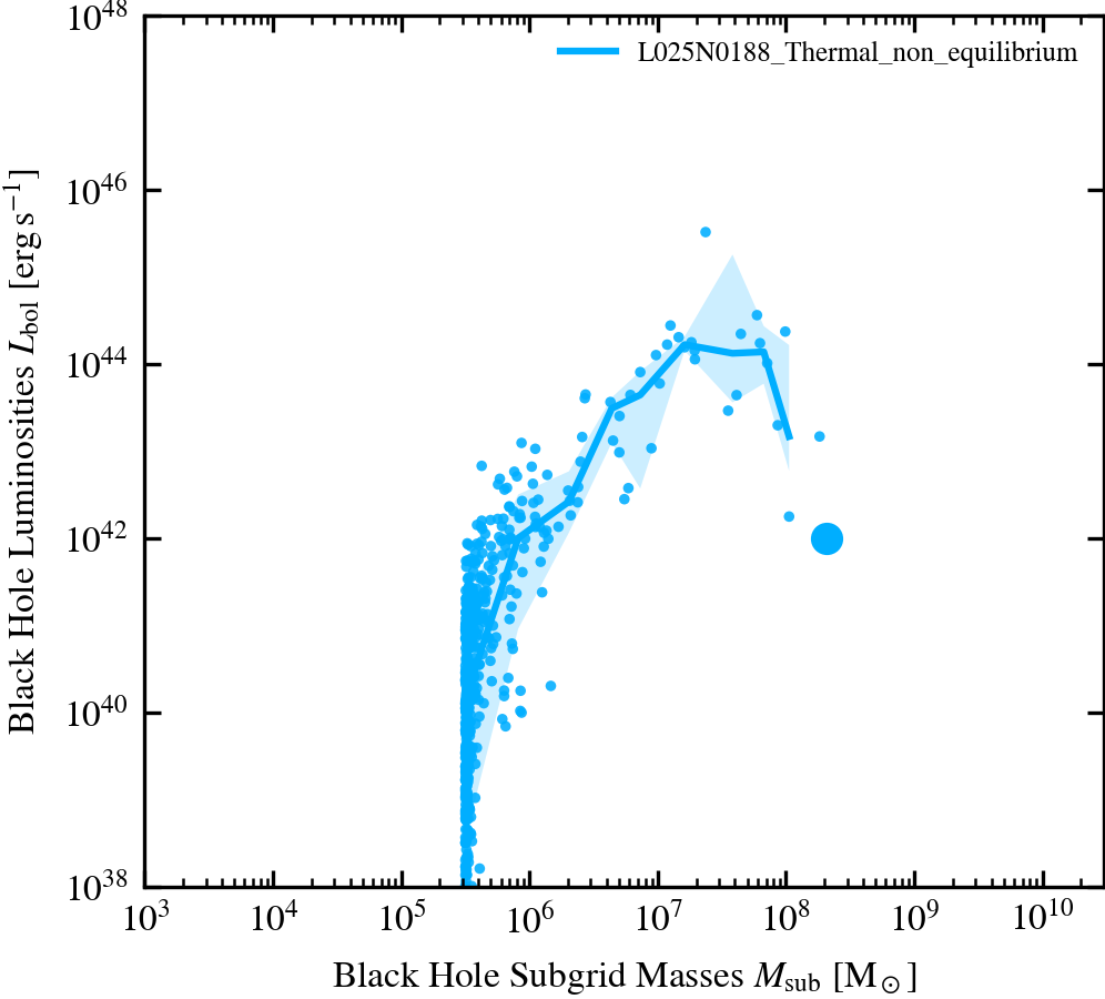
Black Hole Luminosity - Mass Relation
The (instantaneous and bolometric) AGN luminosity versus subgrid mass. Note that this does not include the coupling efficiency factor, i.e. this is not the thermal heating rate.
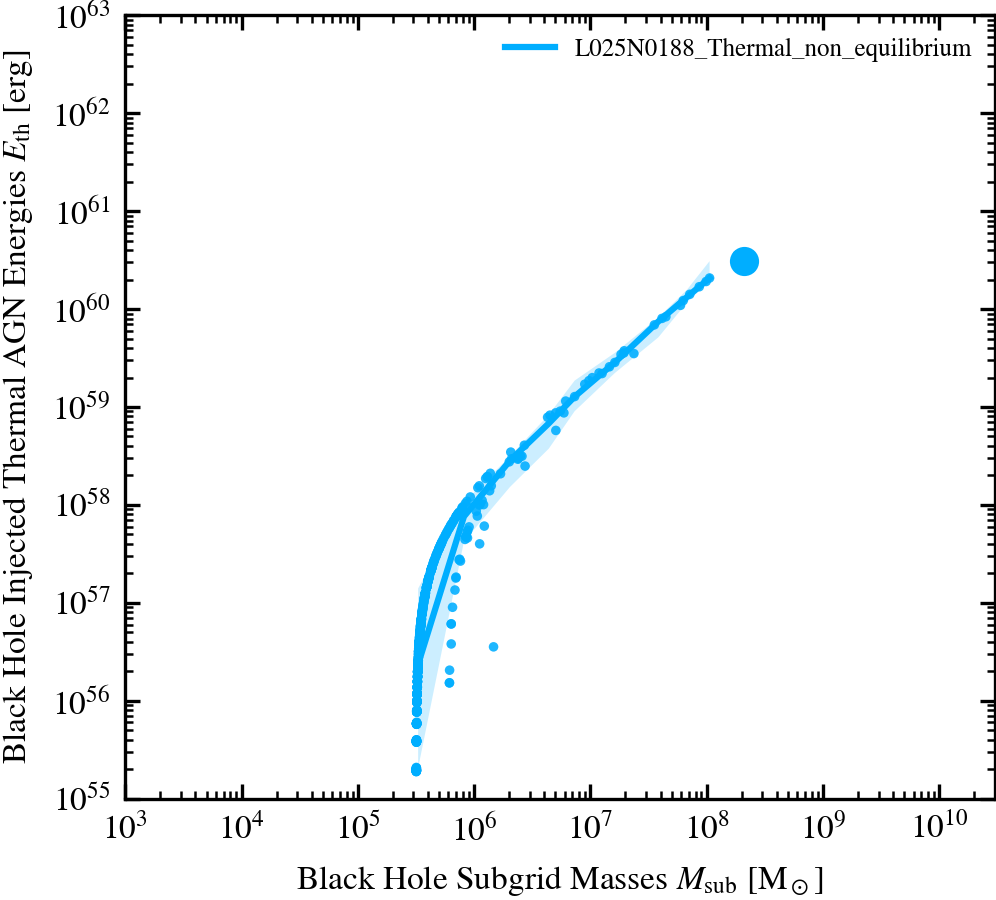
Black Hole Thermal Energy - Mass Relation
The total AGN injected thermal energies (over the BH lifetime) versus subgrid mass.
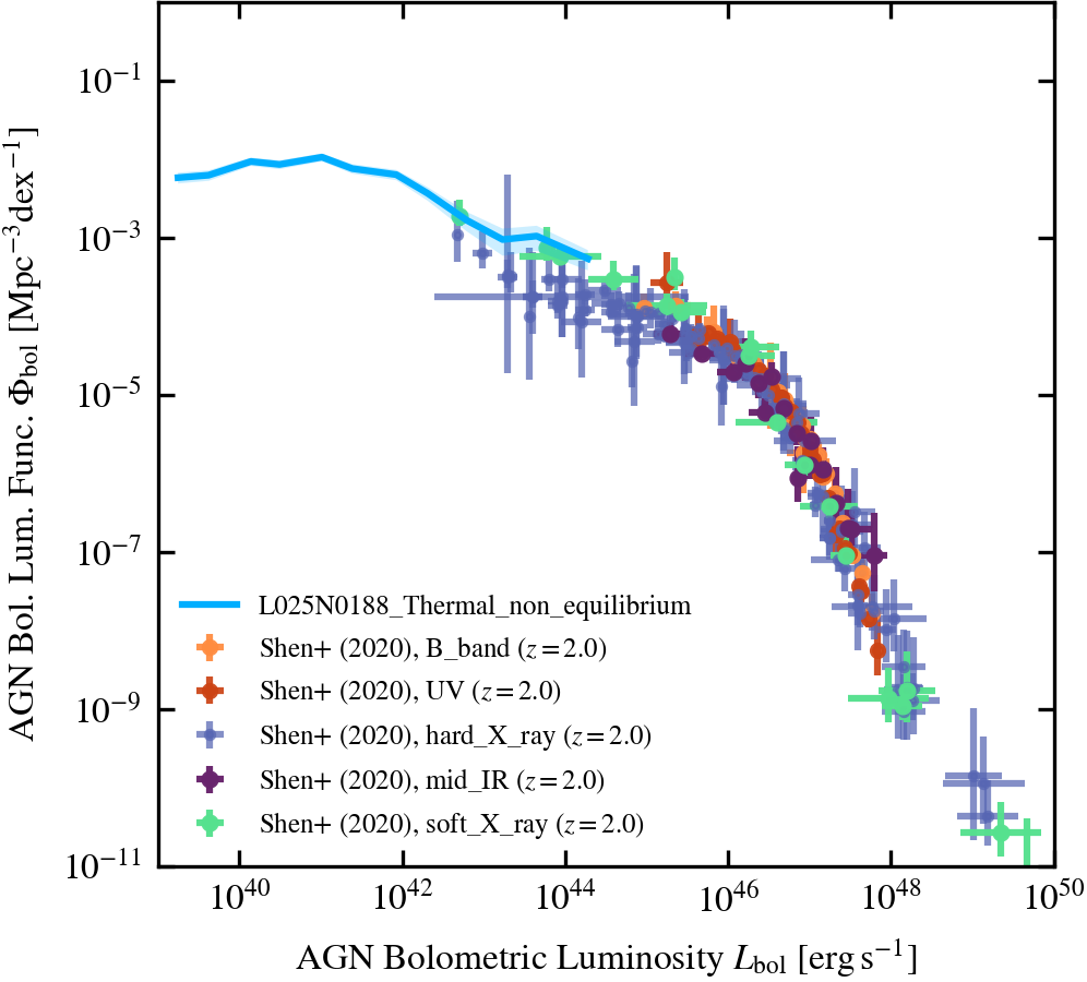
Black Hole AGN Bolometric Luminosity Function
The AGN bolometric luminosity function calculated from the accretion rates and radiative efficiencies. The observational data is inferred from different bands using correction factors.
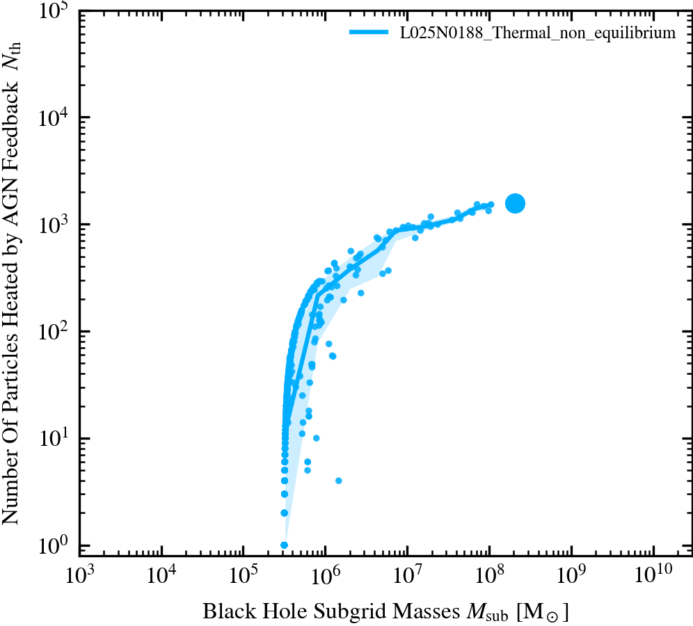
Black Hole AGN Heating Events - Mass Relation
The total number of particles heated by AGN thermal feedback (over the BH lifetime) versus subgrid mass.
Black Holes Evolution
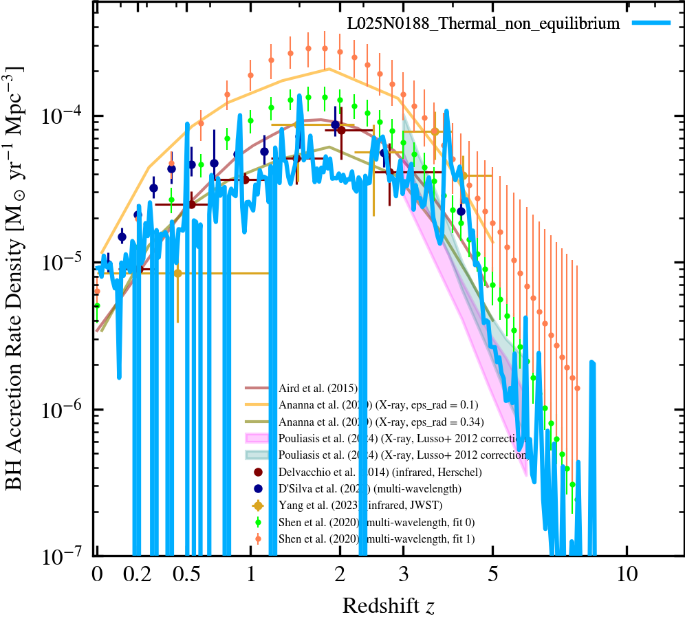
Black Hole Accretion History
Evolution of the accretion rate onto BHs per unit co-moving volume.
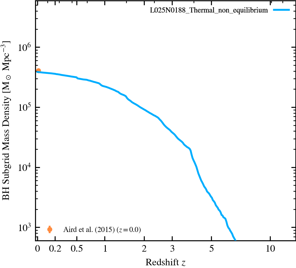
Black Hole Mass History
Evolution of the BH mass per unit co-moving volume.
Cold Gas Data Comparison
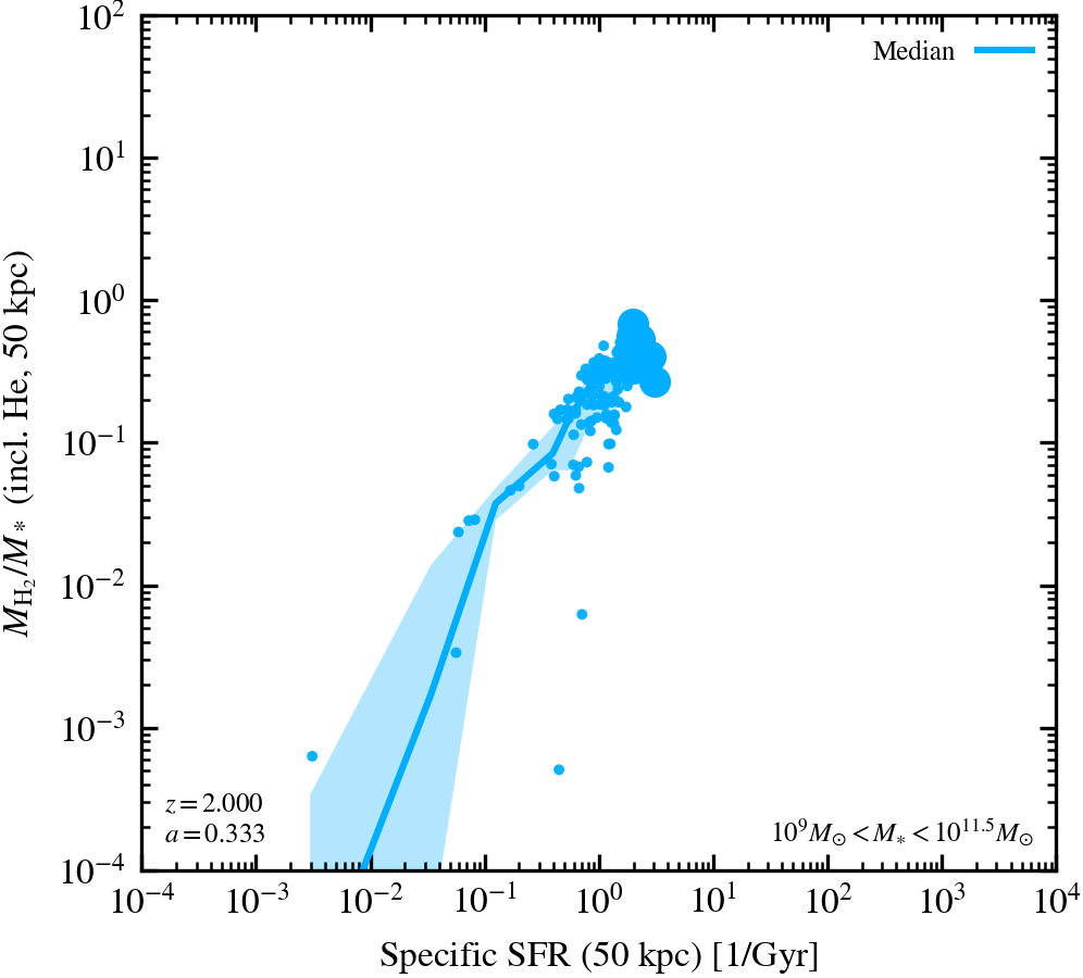
sSFR-H$_2$ Fraction
Galaxy H$_2$ mass (including Helium following the observations) over stellar mass as a function of specific star formation rate in 0.2 dex bins, measured in 50 kpc apertures. To include Helium we multiply $M_{\rm H_2}/M_{\rm star}$ by $(1+M_{\rm He}/M_{\rm H})$. The median values are shown.
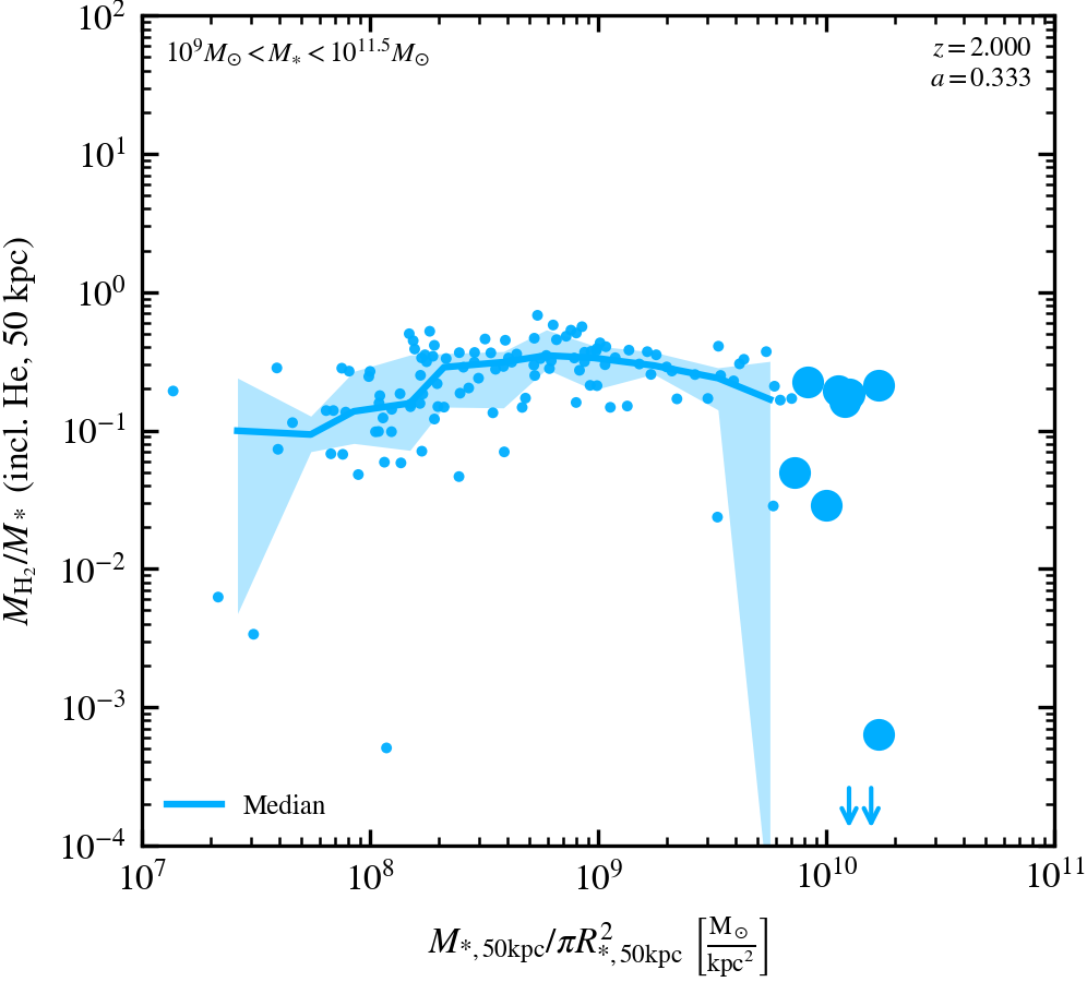
Stellar Mass Surface Density-H$_2$ Fraction
Galaxy H$_2$ mass (including Helium following the observations) over stellar mass as a function of stellar mass surfaced density in 0.2 dex bins, measured in 50 kpc apertures. To include Helium we multiply $M_{\rm H_2}/M_{\rm star}$ by $(1+M_{\rm He}/M_{\rm H})$. The median values are shown.
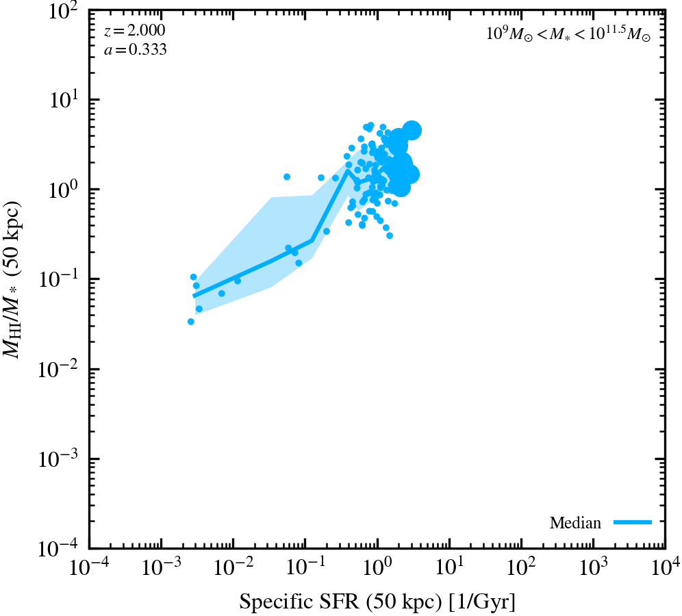
sSFR-HI Fraction
Galaxy HI mass over stellar mass as a function of specific star formation rate in 0.2 dex bins, measured in 50 kpc apertures. XGASS (Catinella+18) galaxies are selected to have a flat $M_\star$ distribution in the range $10^9 \; {\rm M_\odot} > M_\star > 10^{10} \; {\rm M_\odot}$, and a higher normalised uniform in the range $10^{10} \; {\rm M_\odot} > M_\star > 10^{11} \; {\rm M_\odot}$.
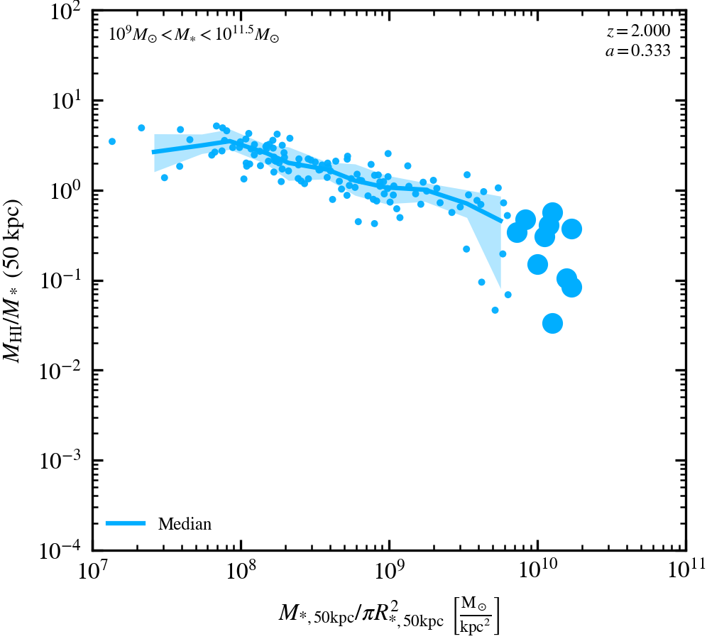
Stellar Mass Surface Density-HI Fraction
Galaxy HI mass over stellar mass as a function of stellar mass surface density in 0.2 dex bins, measured in 50 kpc apertures. XGASS (Catinella+18) galaxies are selected to have a flat $M_\star$ distribution in the range $10^9 \; {\rm M_\odot} > M_\star > 10^{10} \; {\rm M_\odot}$, and a higher normalised uniform in the range $10^{10} \; {\rm M_\odot} > M_\star > 10^{11} \; {\rm M_\odot}$.
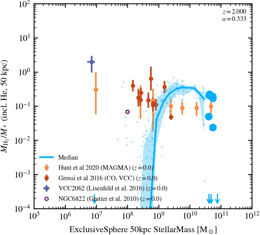
Stellar Mass-H$_2$ Fraction
Galaxy H$_2$ mass (including Helium following the observations) over stellar mass as a function of stellar mass in 0.2 dex bins, measured in 50 kpc apertures. To include Helium we multiply $M_{\rm H_2}/M_{\rm star}$ by $(1+M_{\rm He}/M_{\rm H})$. The median values are shown. In Saintonge2017+ data, all galaxies with $10^9 < M_{\rm star} / \mathrm{M_\odot} < 10^{10}$ have $M_{\rm H_2}/M_{\rm star}$ fractions that cannot be lower than $0.025$, and for galaxies with $M_{\rm star} / \mathrm{M_\odot} > 10^{10}$ the floor value is $0.015$. The median values ("Binning") are shown.
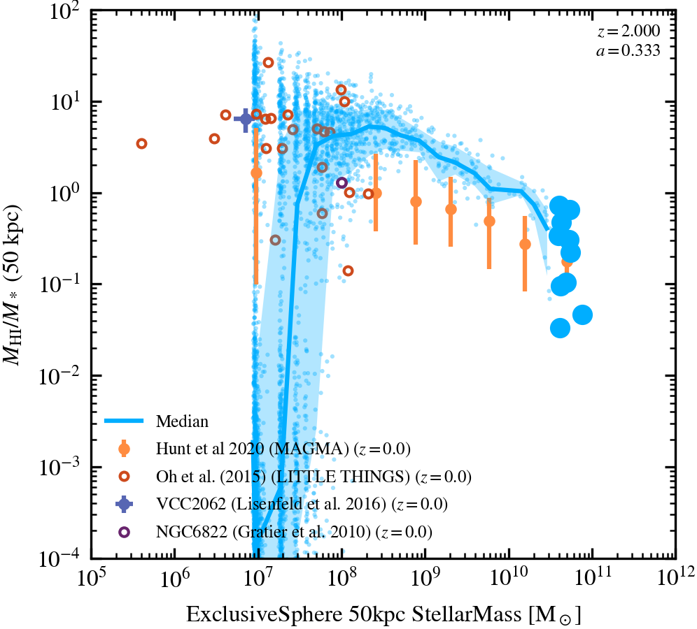
Stellar Mass-HI Fraction
Galaxy HI mass over stellar mass as a function of stellar mass in 0.2 dex bins, measured in 50 kpc apertures. LITTLE THINGS galaxies are dIrrs selected to be within 10 Mpc, with 50$\%$ of galaxies within 3.6 Mpc, and detected in HI. MAGMA (Hunt+20) are selected on both CO and HI detecions, but find the galaxies down to $10^7 \; {\rm M_\odot}$ consistent with the extrapolated SFMS (i.e. typical star-forming galaxies). XGASS (Catinella+18) galaxies are selected to have a flat $M_\star$ distribution in the range $10^9 \; {\rm M_\odot} > M_\star > 10^{10} \; {\rm M_\odot}$, and a higher normalised uniform in the range $10^{10} \; {\rm M_\odot} > M_\star > 10^{11} \; {\rm M_\odot}$.
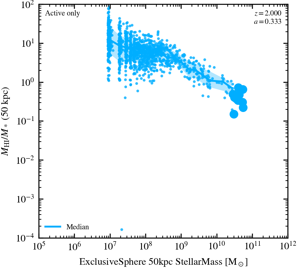
Stellar Mass-HI Fraction (active galaxies)
Galaxy HI mass over stellar mass as a function of stellar mass in 0.2 dex bins, measured in 50 kpc apertures. Active galaxies only.
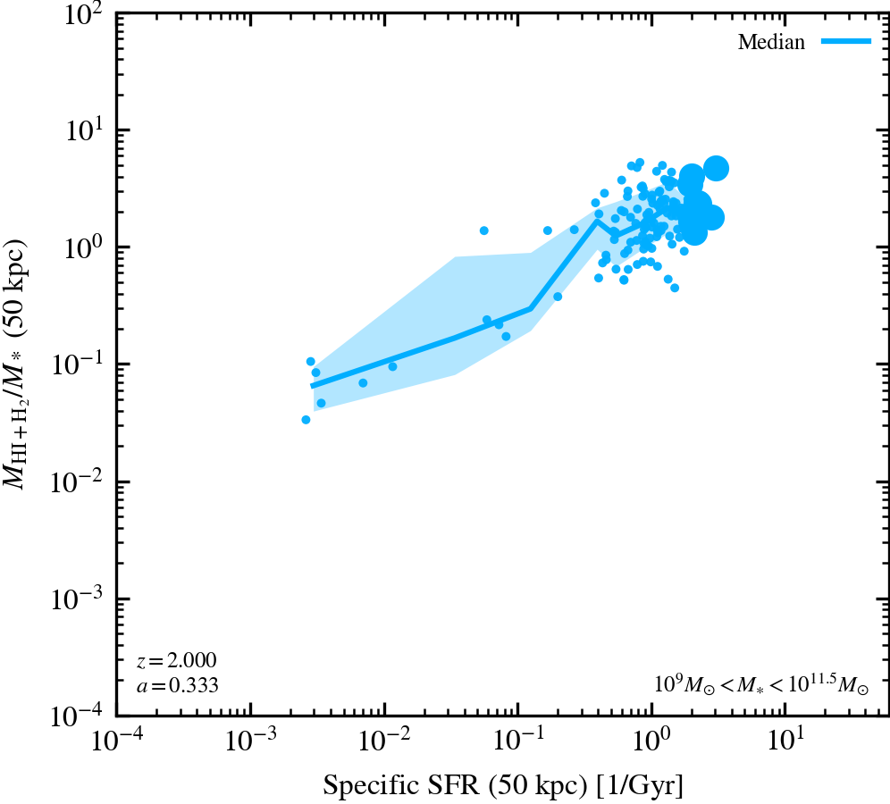
sSFR-Cold gas Fraction
Galaxy neutral gas mass over stellar mass as a function of specific star formation rate, with adaptive binning, measured in 50 kpc apertures. XGASS (Catinella+18) galaxies are selected to have a flat $M_\star$ distribution in the range $10^9 \; {\rm M_\odot} > M_\star > 10^{10} \; {\rm M_\odot}$, and a higher normalised uniform in the range $10^{10} \; {\rm M_\odot} > M_\star > 10^{11} \; {\rm M_\odot}$.
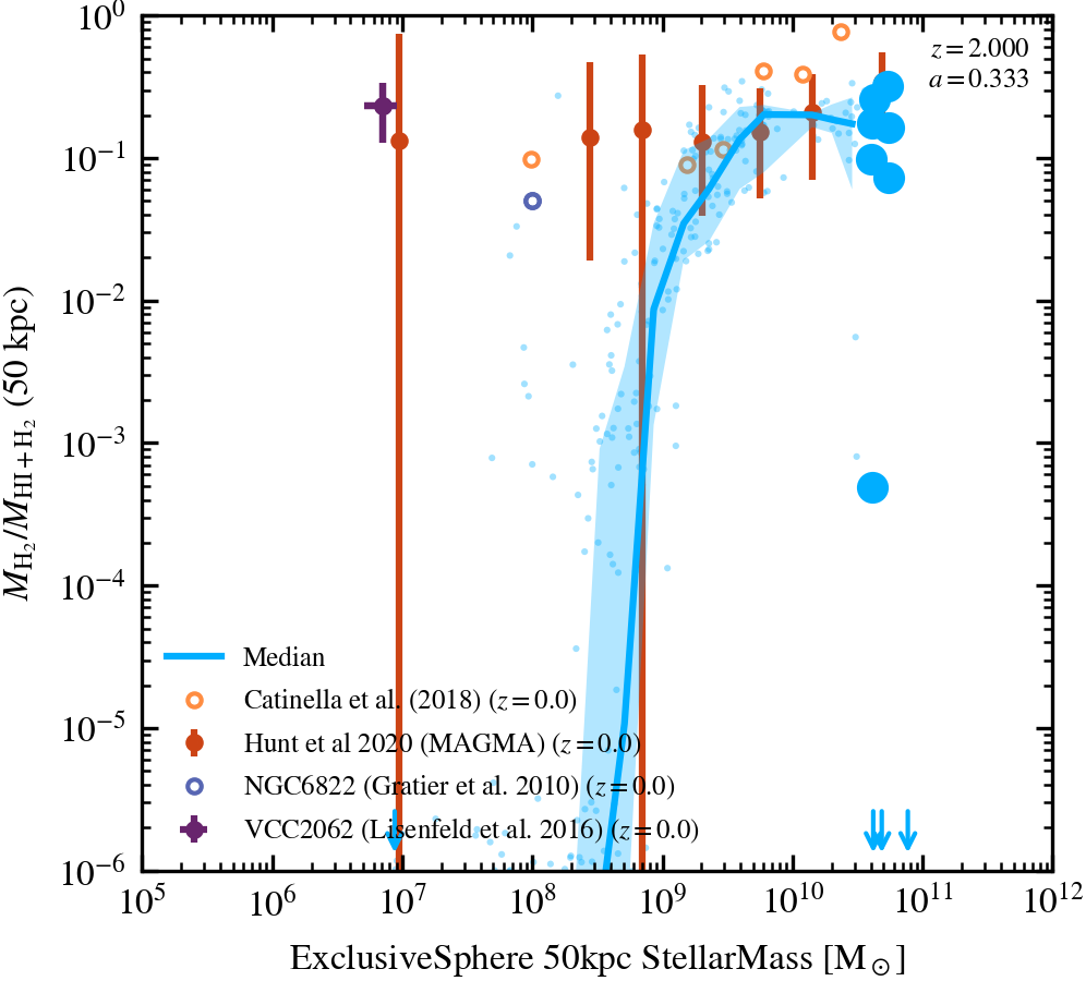
Stellar Mass-Cold gas Fraction
Galaxy H$_2$ mass over neutral gas (HI+H$_2$) mass as a function of stellar mass in 0.2 dex bins, measured in 50 kpc apertures. MAGMA (Hunt+20) are selected on both CO and HI detecions, but find the galaxies down to $10^7 \; {\rm M_\odot}$ consistent with the extrapolated SFMS (i.e. typical star-forming galaxies). XGASS and XCOLDGASS samples are uniform in mass in the range $10^9 \; {\rm M_\odot} > M_\star > 10^{10} \; {\rm M_\odot}$ and $10^{10} \; {\rm M_\odot} > M_\star > 10^{11} \; {\rm M_\odot}$ and plotting those above the CO detection limit ($M_{\rm H2}/M_*$ > $1.5\%$).
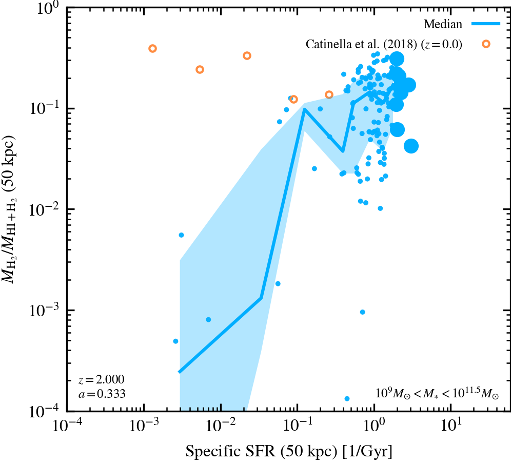
sSFR-Neutral Fraction
Galaxy H$_2$ mass over neutral gas mass (HI+H$_2$) as a function of specific star formation rate, with adaptive binning, measured in 50 kpc apertures. XCOLDGASS (Saintonge+17) and XGASS (Catinella+18) galaxies are selected to have a flat $M_\star$ distribution in the range $10^9 \; {\rm M_\odot} > M_\star > 10^{10} \; {\rm M_\odot}$, and a higher normalised uniform in the range $10^{10} \; {\rm M_\odot} > M_\star > 10^{11} \; {\rm M_\odot}$.
Cold Gas Evolution
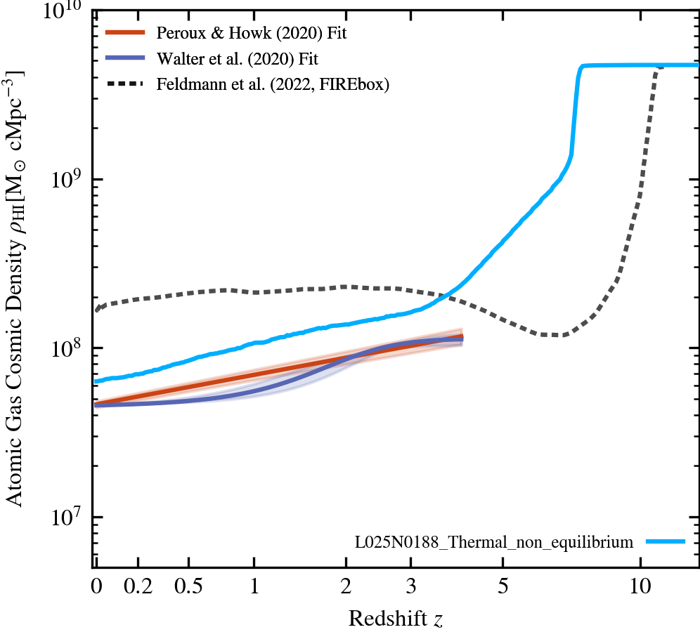
Atomic Gas Mass Evolution
Evolution of the atomic gas mass abundance plotted directly from the statistics.txt file produced by SWIFT, compared with assorted observational estimates corrected to our cosmology. The simulation data is corrected for Helium by multiplying it by 1/0.76.
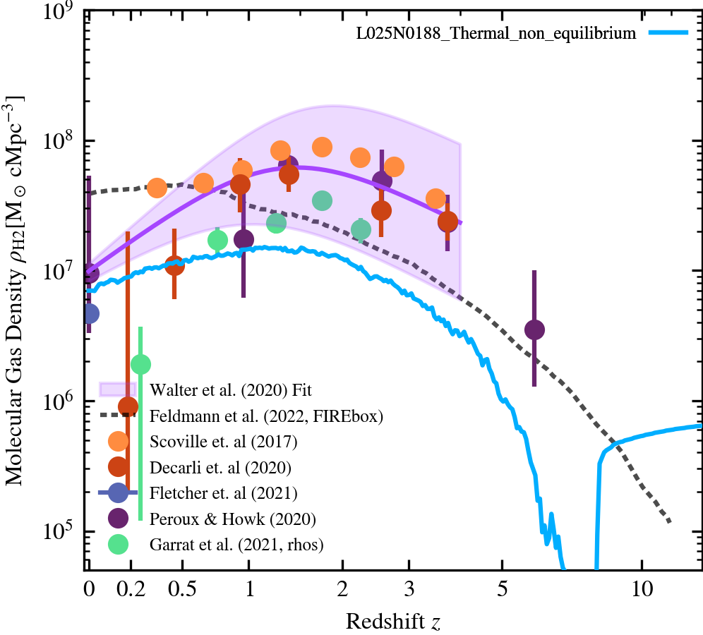
Molecular Gas Mass Evolution
Evolution of the molecular gas mass abundance plotted directly from the statistics.txt file produced by SWIFT, compared with assorted observational estimates.
Cold Gas Fractions (sSFR)
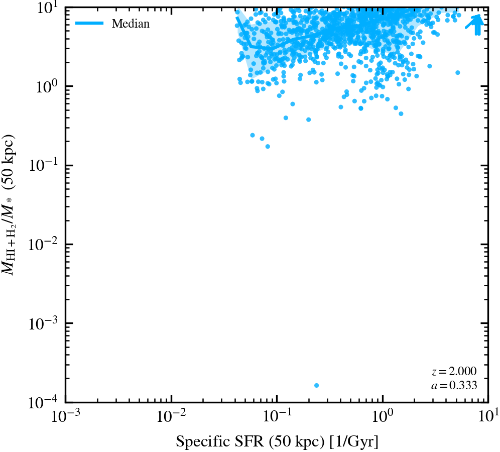
sSFR-Neutral Gas to SF Gas Fraction (50 kpc aperture)
Only active galaxies are included in the median line. Fraction is HI + H$_2$ mass over stellar mass in a 50 kpc aperture.
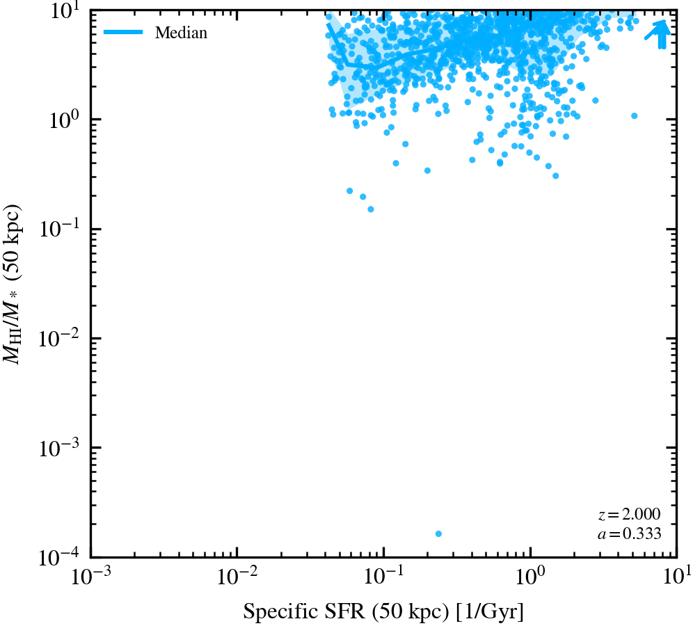
sSFR-HI Gas to SF Gas Fraction (50 kpc aperture)
Only active galaxies are included in the median line. Fraction is HI mass over stellar mass in a 50 kpc aperture.
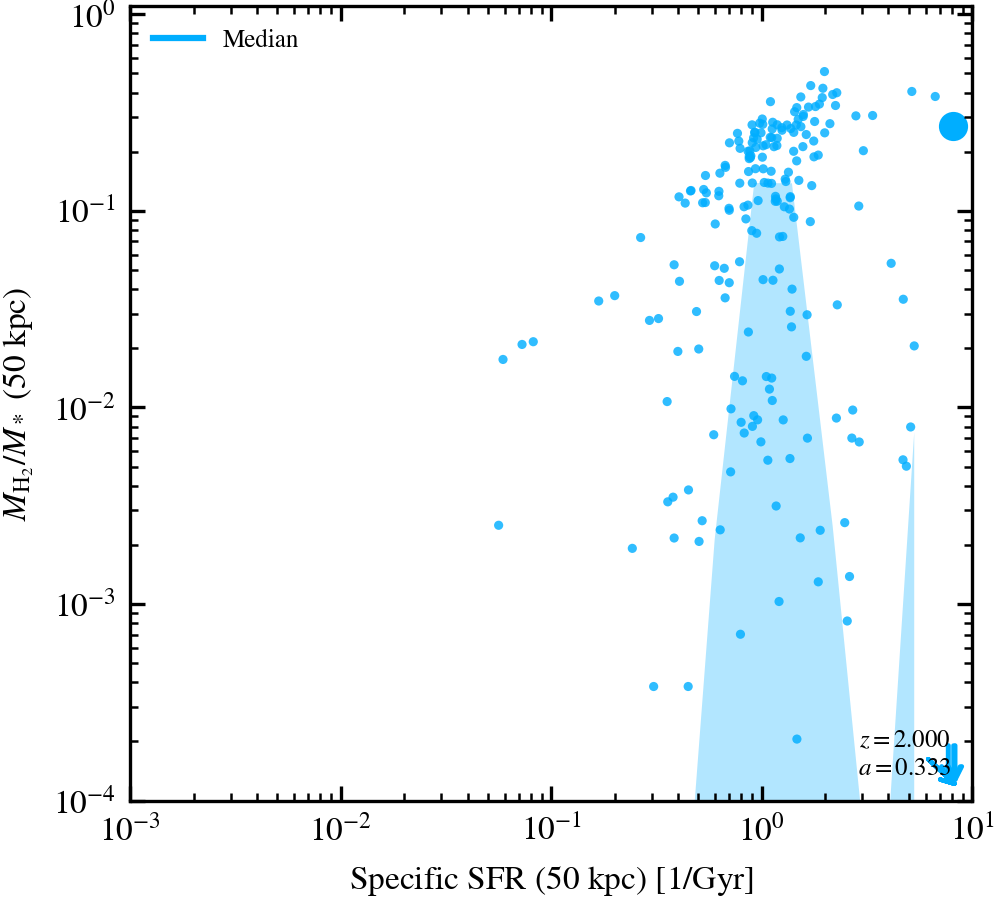
sSFR-H$_2$ Gas to SF Gas Fraction (50 kpc aperture)
Only active galaxies are included in the median line. Fraction is H$_2$ mass over stellar mass in a 50 kpc aperture.
Cold Gas Fractions (Stellar Mass)
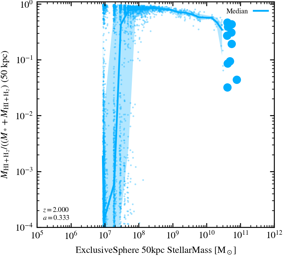
Stellar Mass-Neutral Gas to Baryonic Fraction (50 kpc aperture)
All galaxies are included in the median line. Fraction is HI + H$_2$ mass over total baryonic mass in a 50 kpc aperture.
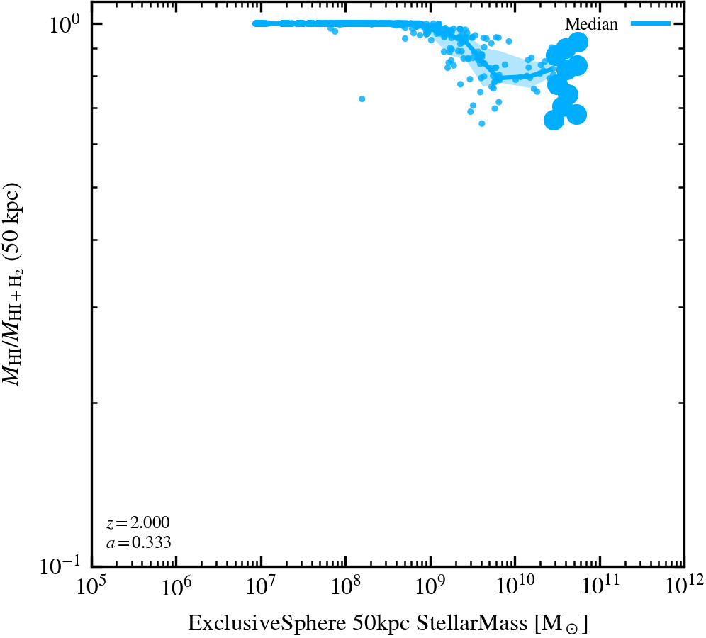
Stellar Mass-HI to Neutral Gas Fraction (50 kpc aperture)
Only active galaxies are included in the median line. Fraction is HI mass over HI + H$_2$ mass in a 50 kpc aperture.
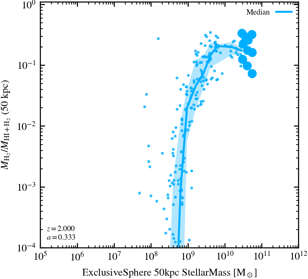
Stellar Mass-H$_2$ to Neutral Gas Fraction (50 kpc aperture)
Only active galaxies are included in the median line. Fraction is H$_2$ mass over HI + H$_2$ mass in a 50 kpc aperture.
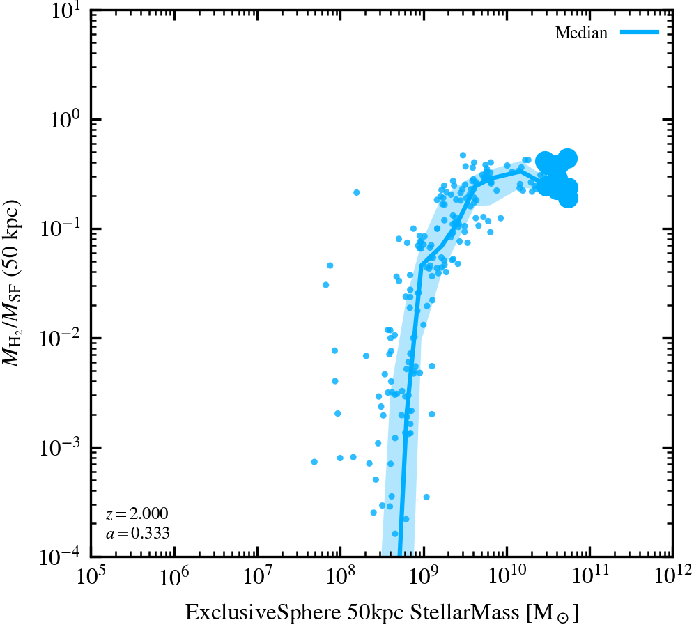
Stellar Mass-H$_2$ to SF Gas Fraction (50 kpc aperture)
Only active galaxies are included in the median line. Fraction is H$_2$ gas mass over SF gas in a 50 kpc aperture.
Cold Gas Masses
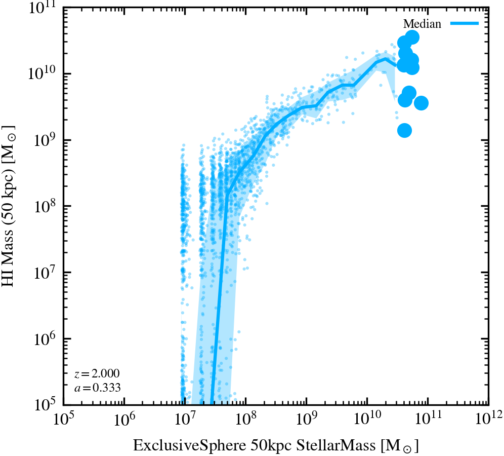
Stellar Mass-HI Gas Mass Relation (50 kpc aperture)
All galaxies are included in the median line. Both stellar and HI masses were computed in 50 kpc apertures.
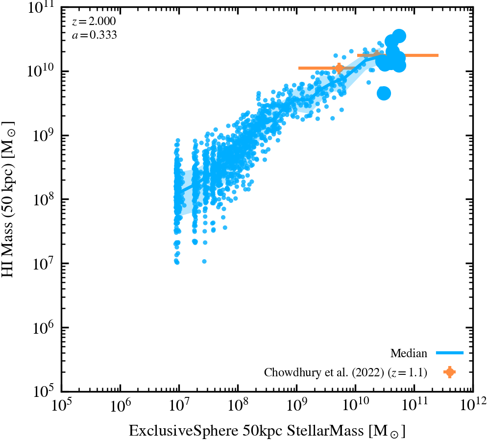
Stellar Mass-HI Gas Mass Relation (50 kpc aperture)
Only active galaxies are included in the median line. Both stellar and HI masses were computed in 50 kpc apertures.
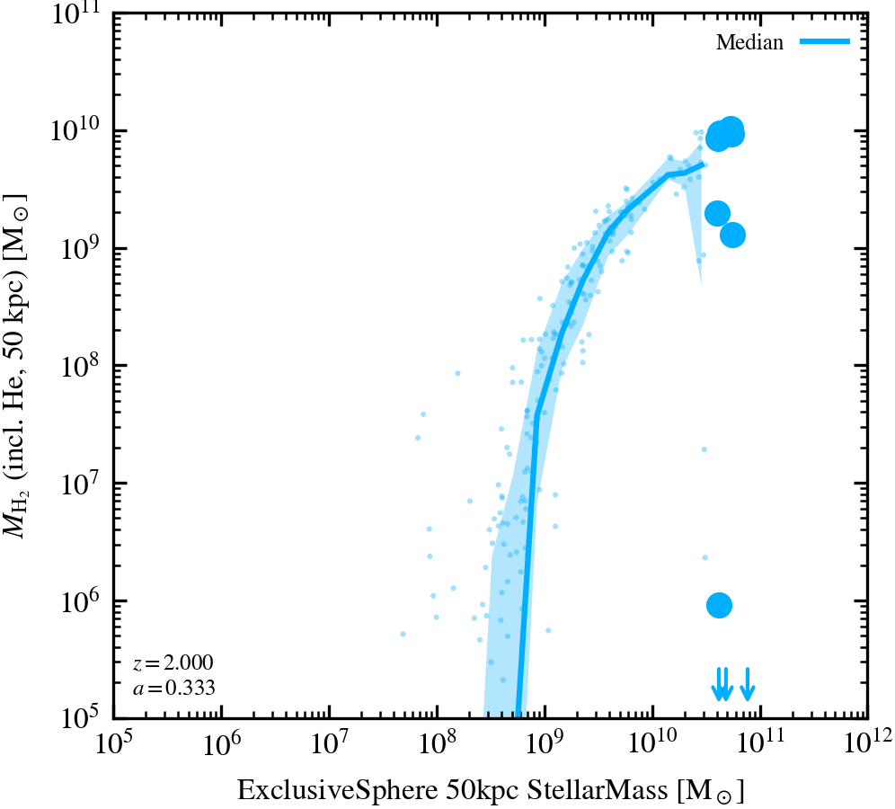
Stellar Mass-H$_2$ Gas Mass Relation (50 kpc aperture)
All galaxies are included in the median line. H$_2$ mass was corrected for Helium. Both stellar and H$_2$ masses were computed in 50 kpc apertures.
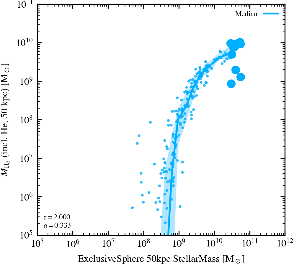
Stellar Mass-H$_2$ Gas Mass Relation (50 kpc aperture)
Only active galaxies are included in the median line. H$_2$ mass was corrected for Helium. Both stellar and H$_2$ masses were computed in 50 kpc apertures.
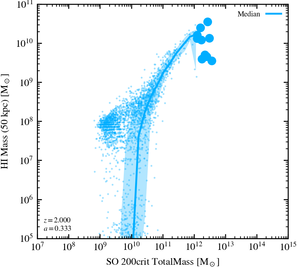
Halo Mass-HI Gas Mass Relation (50 kpc aperture)
All galaxies are included in the median line. HI mass was computed in 50 kpc apertures.
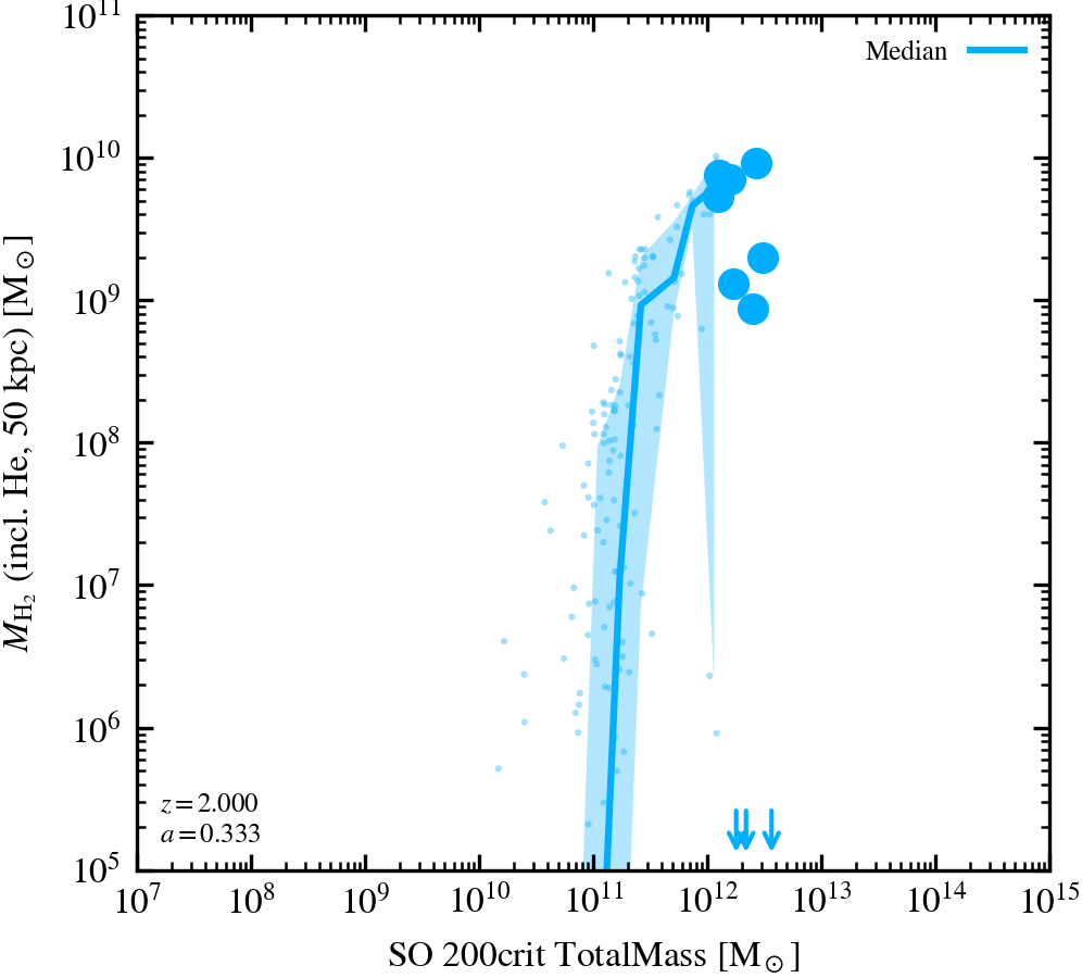
Halo Mass-H$_2$ Gas Mass Relation (50 kpc aperture)
All galaxies are included in the median line. H$_2$ mass was corrected for Helium. H$_2$ mass was computed in 50 kpc apertures.
Column Densities
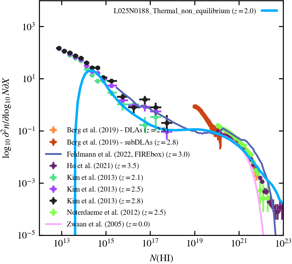
HI Column Density Distribution Function (full box, full range)
The column density distribution function of neutral hydrogen computed by projecting the entire box along the z-axis, corrected for the size of the box in redshift space.
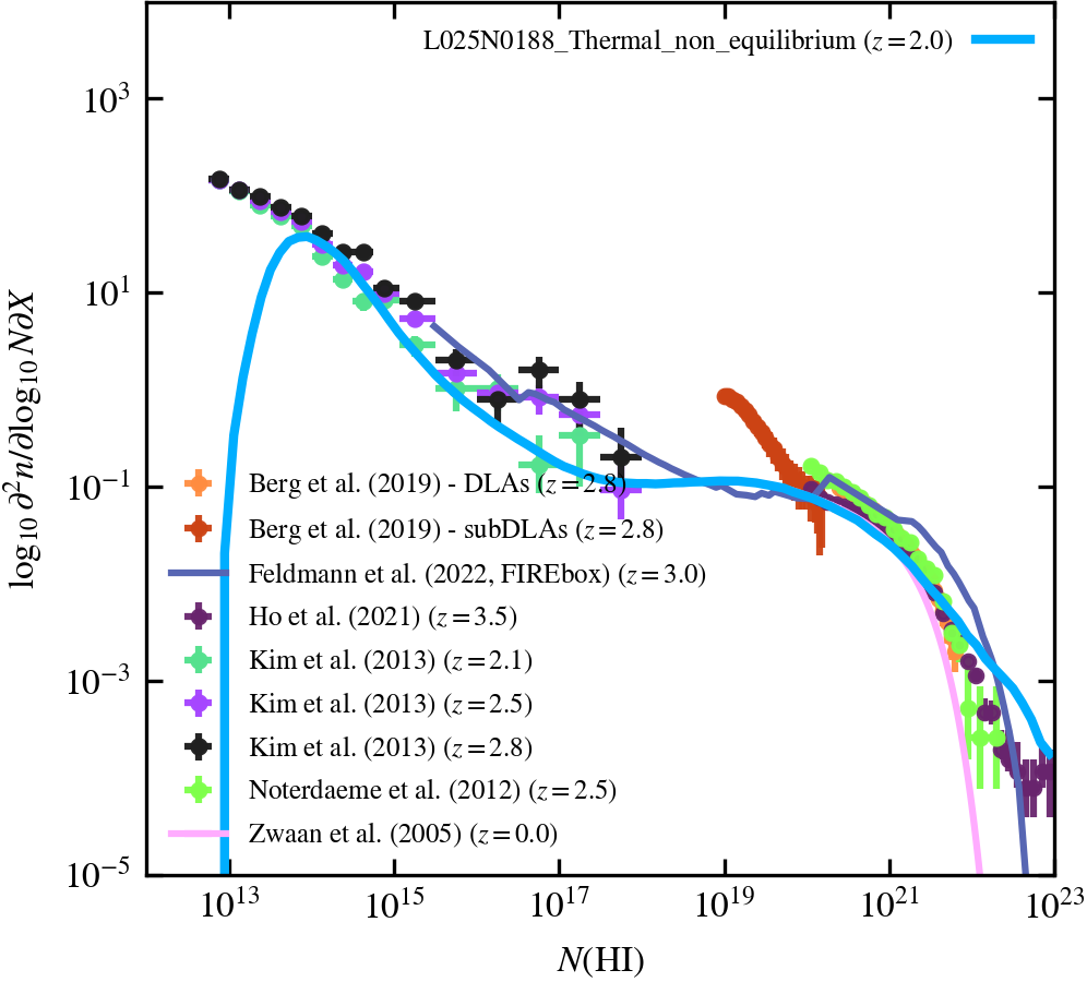
HI Column Density Distribution Function (half box, full range)
The column density distribution function of neutral hydrogen computed by splitting the box in half along the z-axis and projecting each half separately, also along the z-axis. Corrected for the size of the box in redshift space.
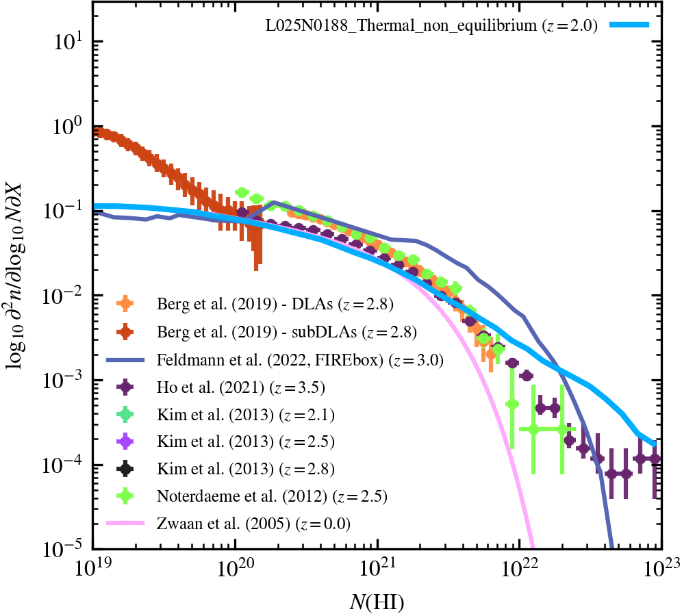
HI Column Density Distribution Function (full box, reduced range)
The column density distribution function of neutral hydrogen computed by projecting the entire box along the z-axis, corrected for the size of the box in redshift space.
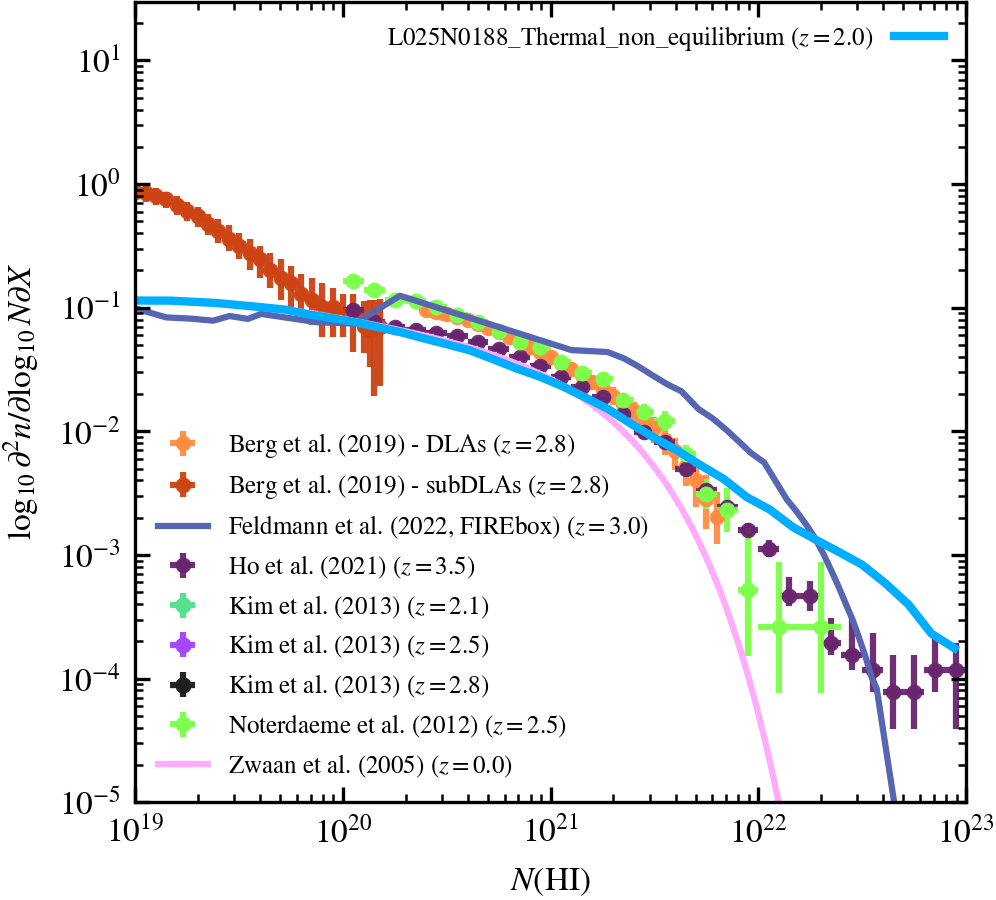
HI Column Density Distribution Function (half box, reduced range)
The column density distribution function of neutral hydrogen computed by splitting the box in half along the z-axis and projecting each half separately, also along the z-axis. Corrected for the size of the box in redshift space.
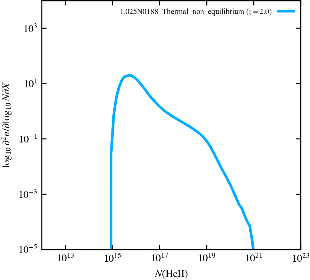
HeII Column Density Distribution Function (full box, full range)
The column density distribution function of singly-ionized helium computed by projecting the entire box along the z-axis, corrected for the size of the box in redshift space.
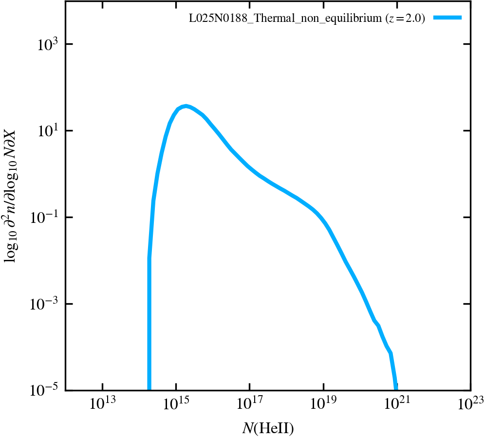
HeII Column Density Distribution Function (half box, full range)
The column density distribution function of singly-ionized helium computed by splitting the box in half along the z-axis and projecting each half separately, also along the z-axis. Corrected for the size of the box in redshift space.
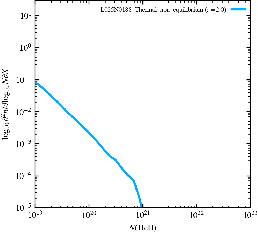
HeII Column Density Distribution Function (full box, reduced range)
The column density distribution function of singly-ionized helium computed by projecting the entire box along the z-axis, corrected for the size of the box in redshift space.
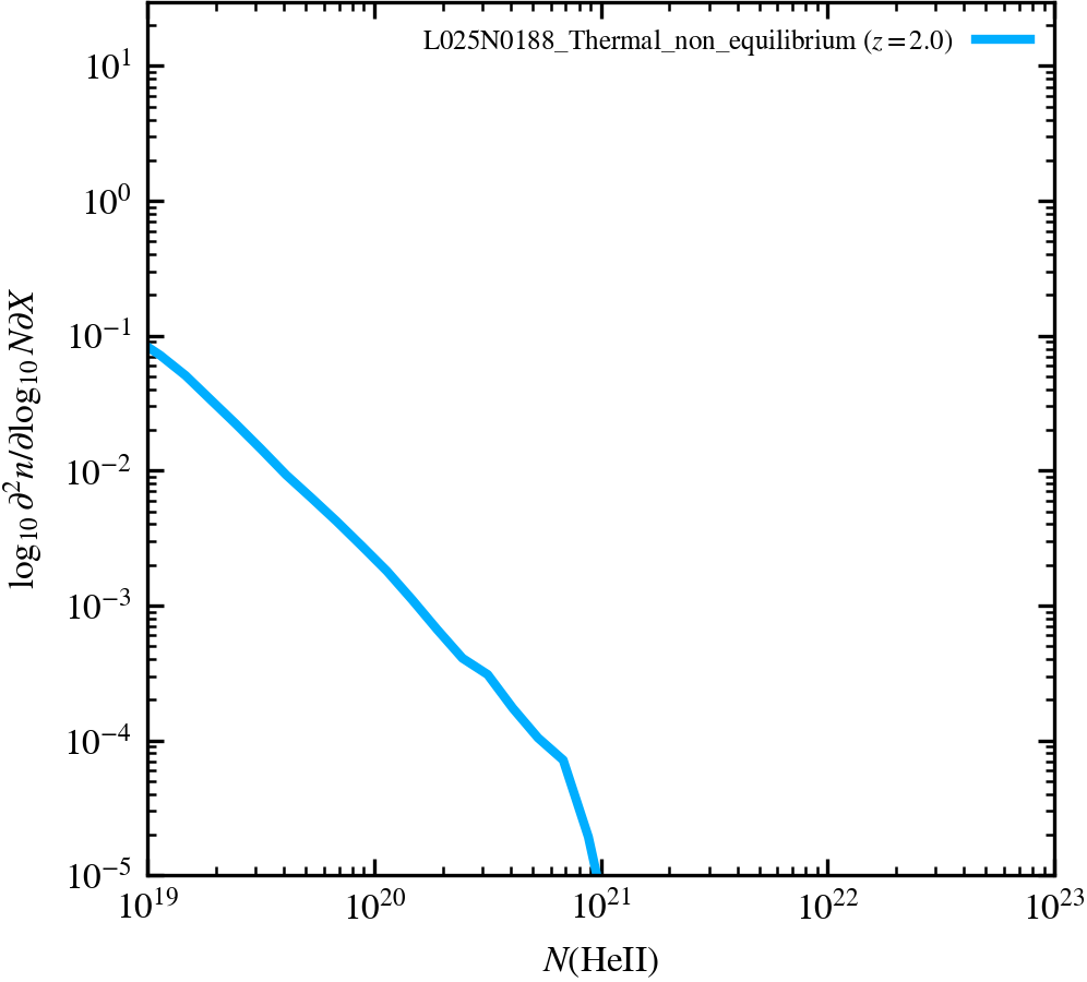
HeII Column Density Distribution Function (half box, reduced range)
The column density distribution function of singly-ionized helium computed by splitting the box in half along the z-axis and projecting each half separately, also along the z-axis. Corrected for the size of the box in redshift space.
Density-Temperature
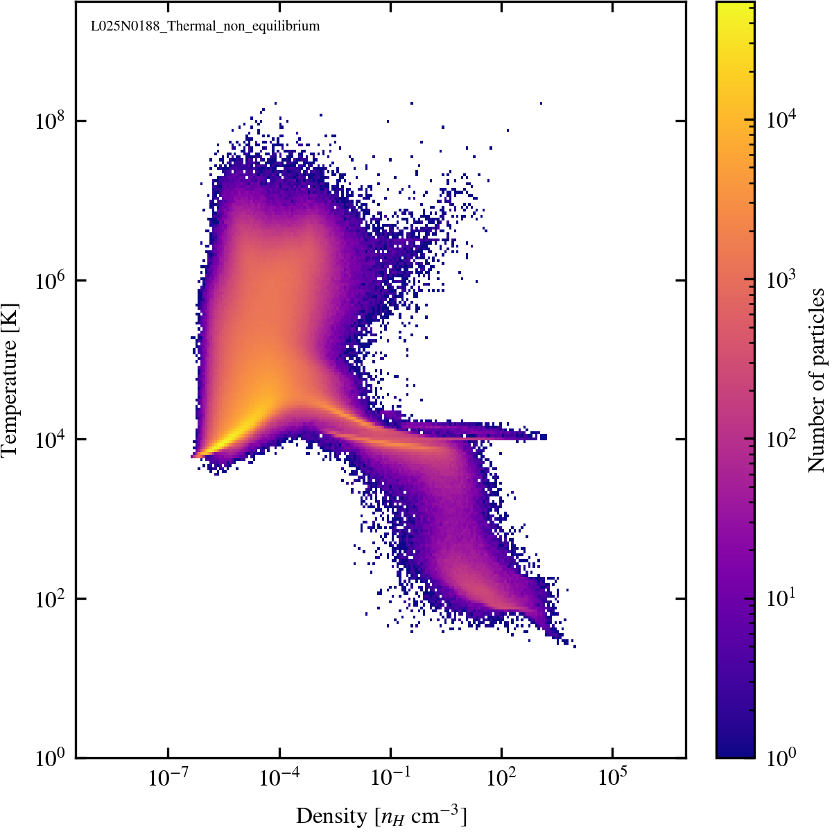
Density-Temperature
Density-temperature diagram. If present, dashed line represents the entropy floor (equation of state).
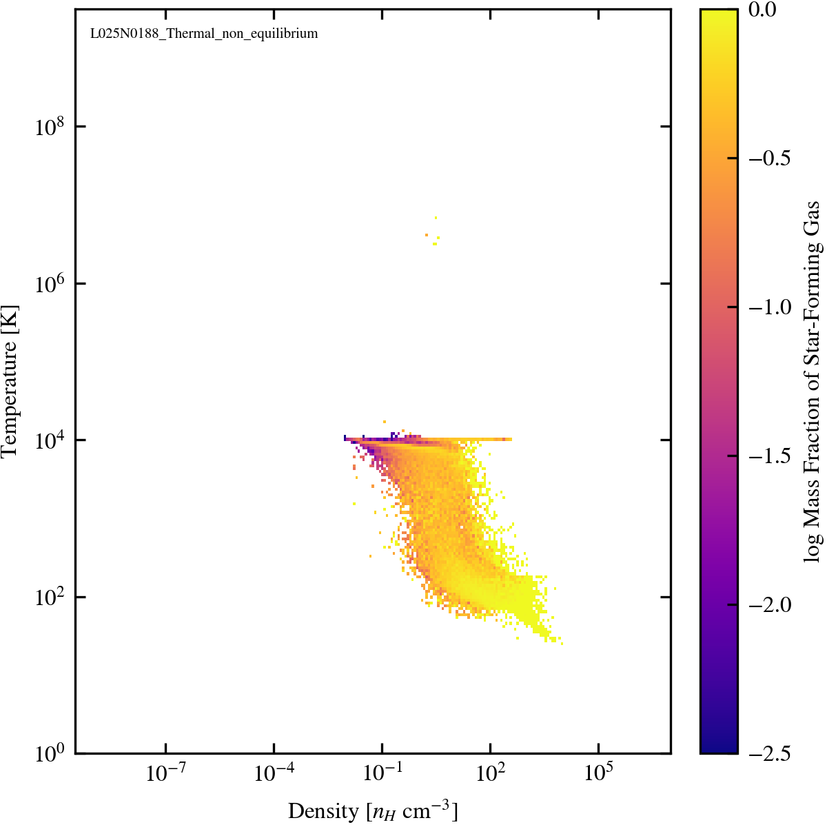
Density-Temperature (Star Forming Gas)
Density-temperature diagram shaded by the mass fraction of the gas whose instantaneous star formation rate is greater than zero.
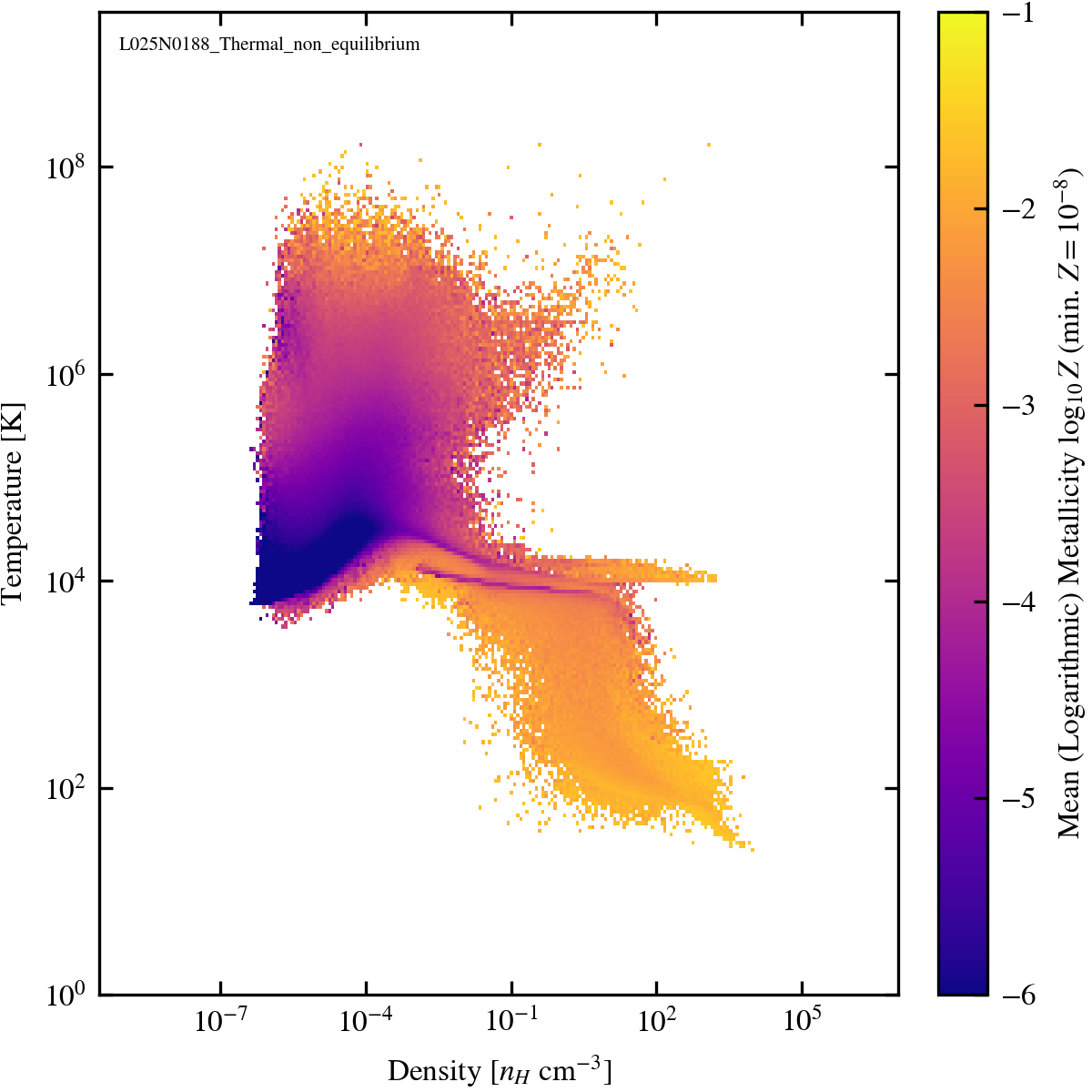
Density-Temperature (Metals)
Density-temperature diagram with the pixel value weighted by the mean logarithmic metal mass fraction (absolute) in that bin. Medians are not used due to their computational complexity. If present, dashed line represents the entropy floor (equation of state).
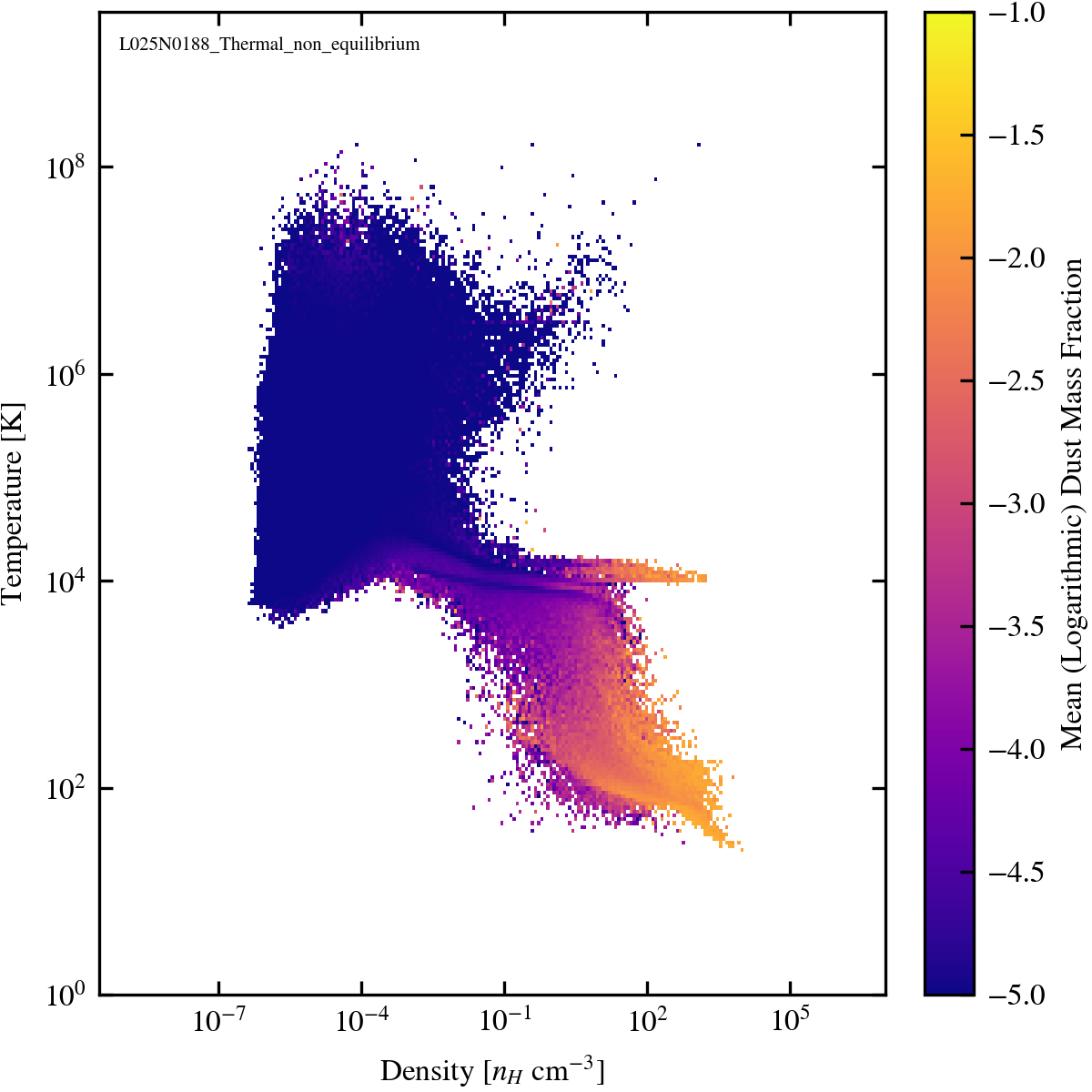
Density-Temperature (Dust)
Density-temperature diagram with the pixel value weighted by the mean logarithmic dust mass fraction in that bin. Medians are not used due to their computational complexity.
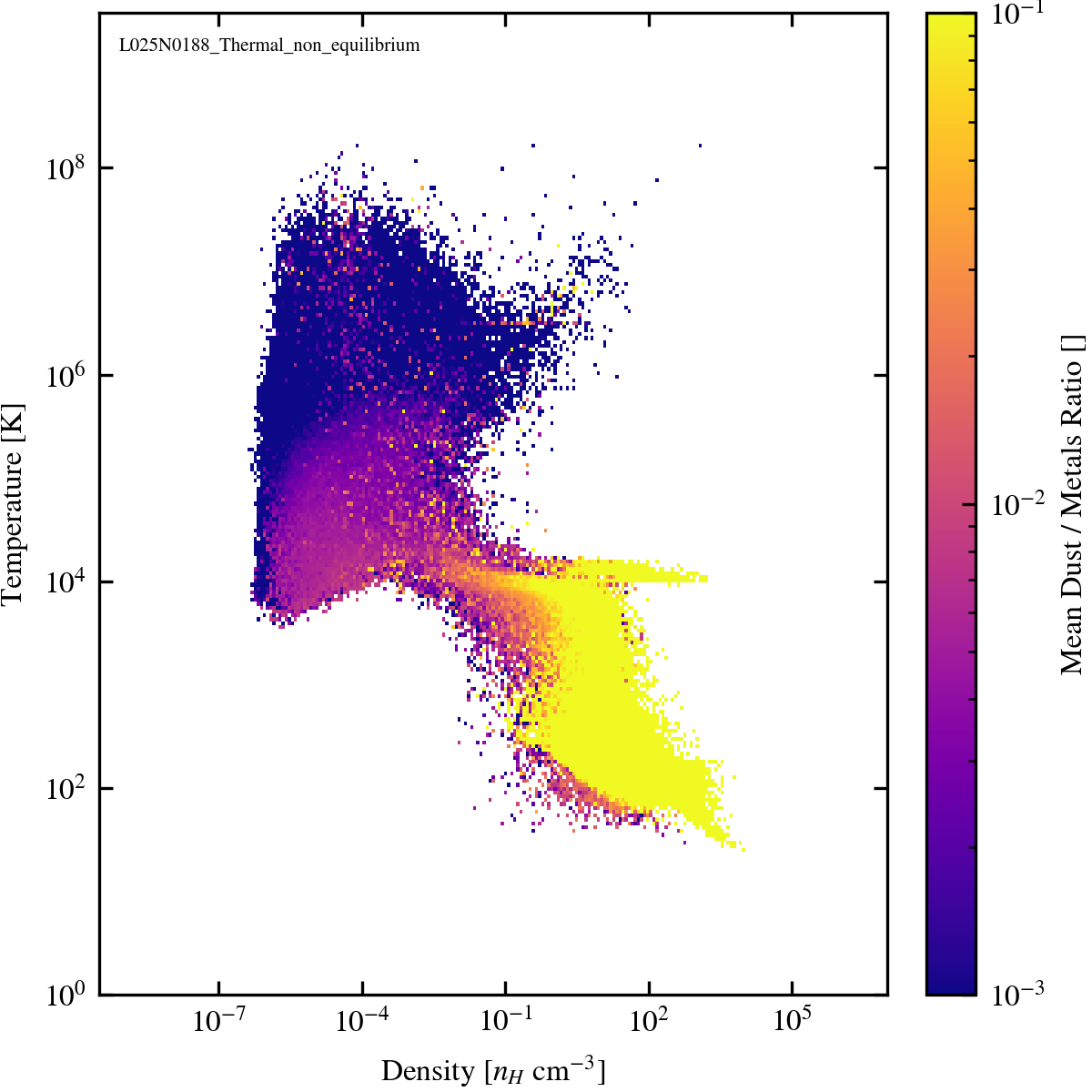
Density-Temperature (Dust / Metals)
Density-temperature diagram with the pixel value the ratio of dust to metals for the particles within that bin (i.e. the values are binned weighted by dust, then by metals, and those two grids are divided to produce the dust to metals ratio). Only particles with a metal mass fraction of $Z > 10^{-8}$ are plotted.
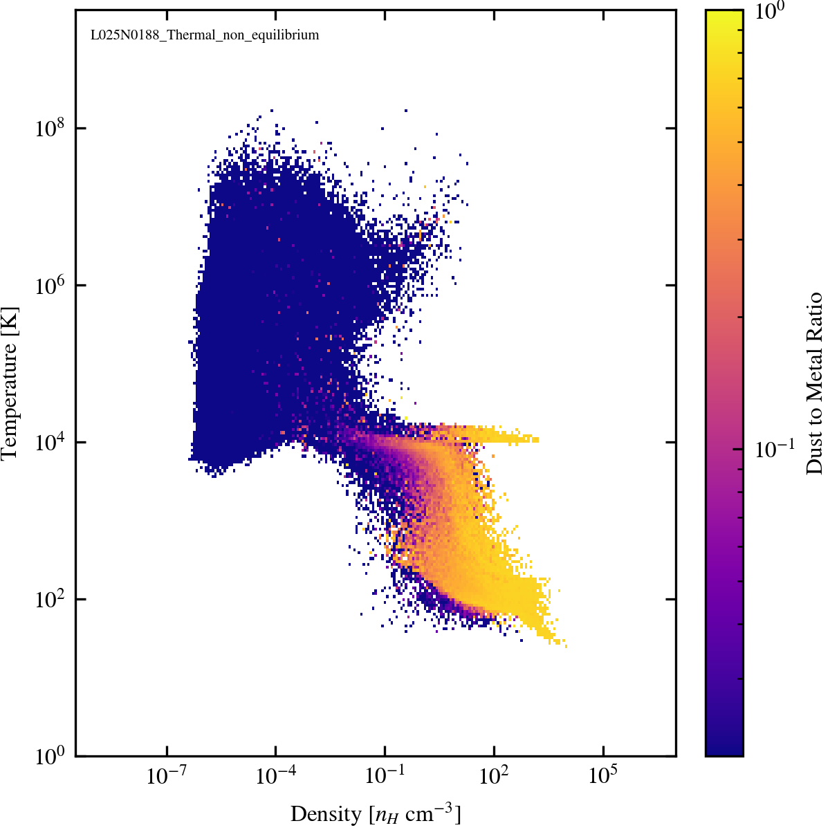
Dust-to-metal Ratio
Density-temperature diagram shaded by the total fraction of metals in the dust phase.
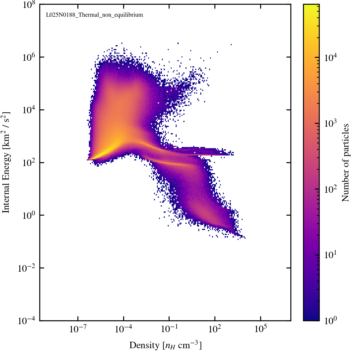
Density-Internal Energy
Density-Internal Energy diagram. If present, dashed line represents the entropy floor (equation of state).
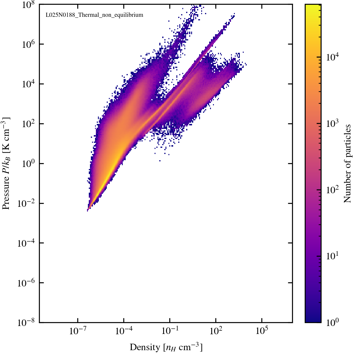
Density-Pressure
Density-pressure diagram. If present, dashed line represents the entropy floor (equation of state).
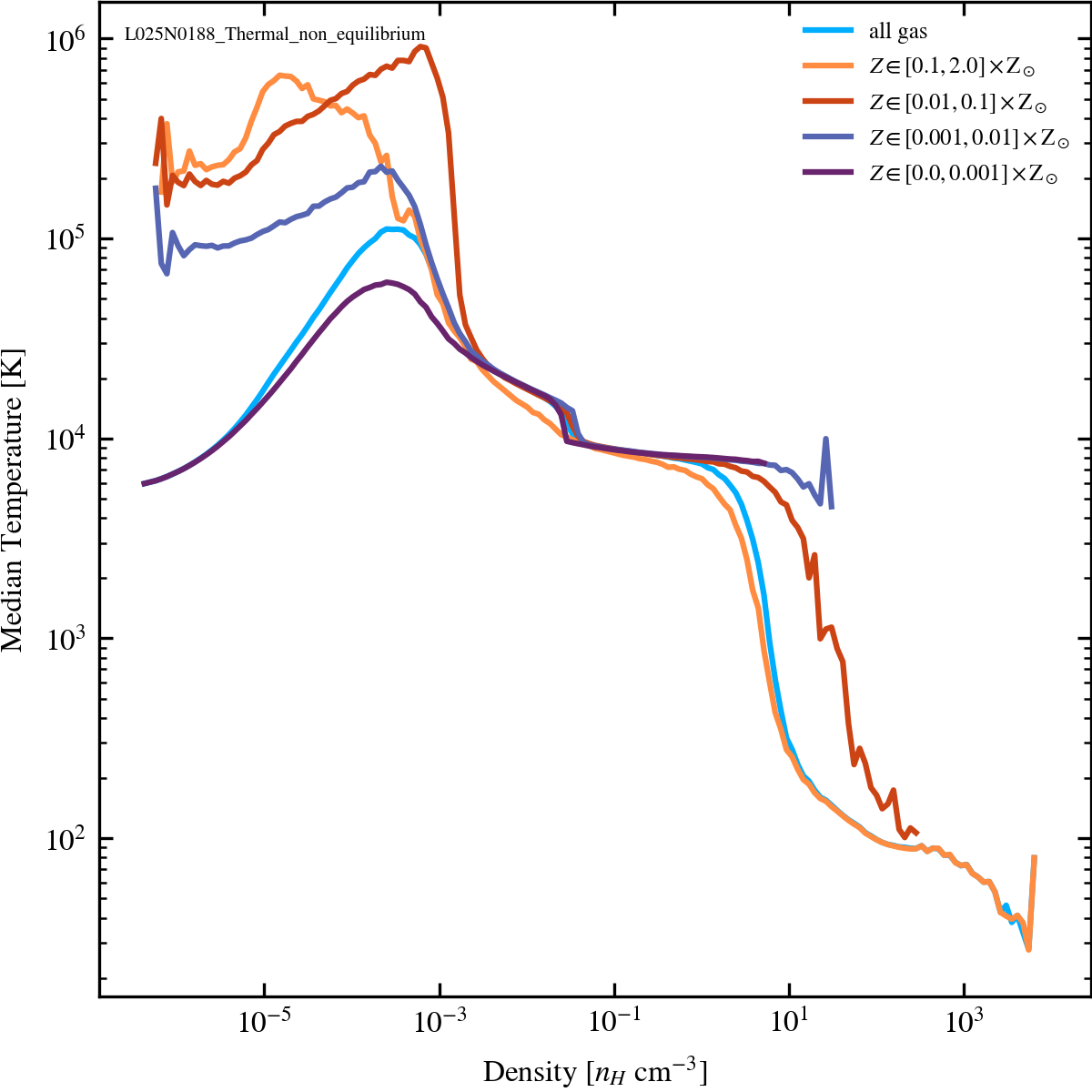
Density-Median Temperature
Median temperature as a function of density for all gas and for gas in selected metallicity ranges.
Dust Depletion Relations
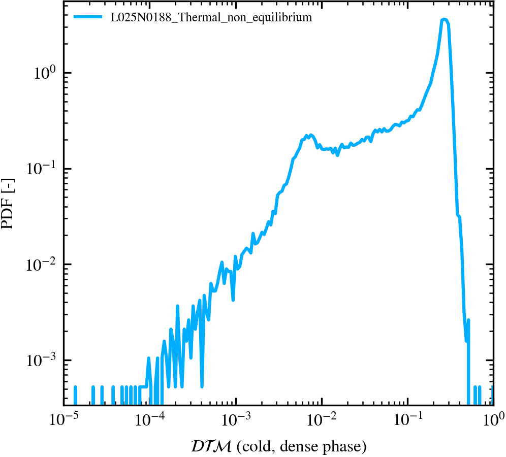
Dust to Metal Ratio
Ratio of dust to metal for cold dense gas.
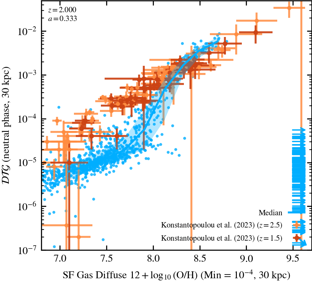
Oxygen abundance vs dust-to-gas ratio in Neutral Gas (30 kpc aperture)
Dust-to-gas mass ratio as a function of oxygen number density abundance in Neutral gas. Only active galaxies are selected.
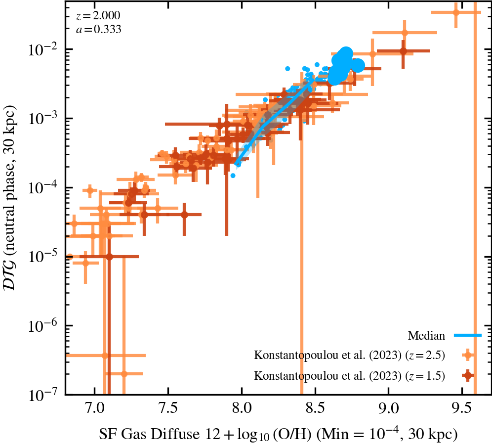
Oxygen abundance vs dust-to-gas ratio in Neutral Gas (30 kpc aperture)
Dust-to-gas mass ratio as a function of oxygen number density abundance in Neutral gas. Only galaxies that are active and have $M_* > 10^9 \, \rm M_\odot$ are selected.
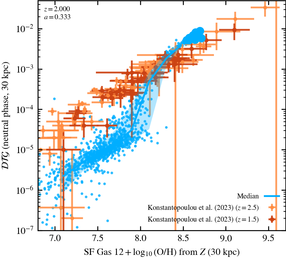
Oxygen abundance (from Z) vs dust-to-gas ratio in Neutral Gas (30 kpc aperture)
Dust-to-gas mass ratio as a function of metallicity represented as an oxygen number density abundance for compatibility with observations. Only active galaxies are selected.
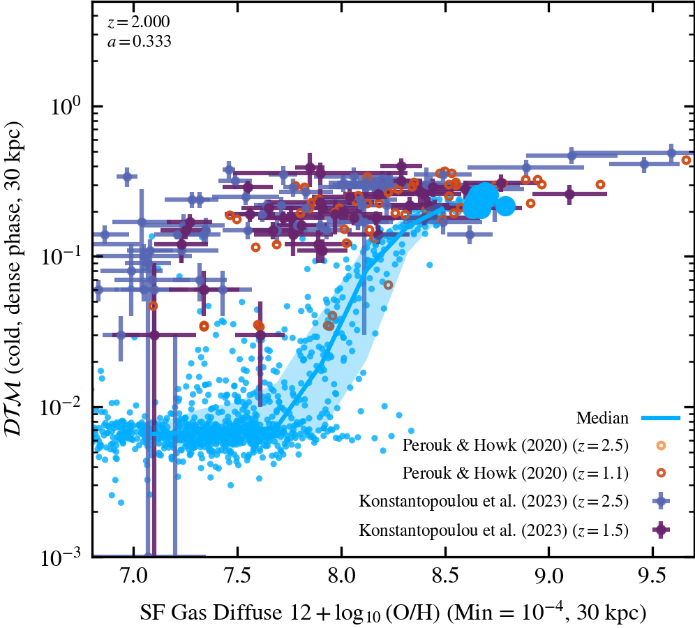
Oxygen abundance vs dust-to-metal ratio in Neutral Gas (30 kpc aperture)
Dust-to-metal mass ratio as a function of oxygen number density abundance in Neutral gas. Only active galaxies are selected.
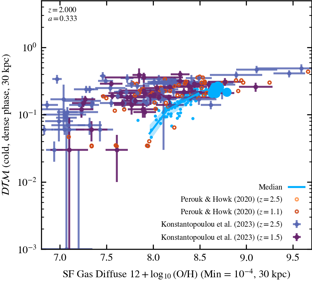
Oxygen abundance vs dust-to-metal ratio in Neutral Gas (30 kpc aperture)
Dust-to-metal mass ratio as a function of oxygen number density abundance in Neutral gas. Only galaxies that are active and have $M_* > 10^9 \, \rm M_\odot$ are selected.
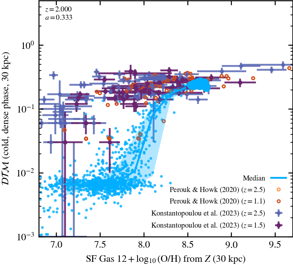
Oxygen abundance (from Z) vs dust-to-metal ratio in Neutral Gas (30 kpc aperture)
Dust-to-metal mass ratio as a function of metallicity, converted into an oxygen number density abundance for compatability with observations. Only active galaxies are selected.
Dust Evolution
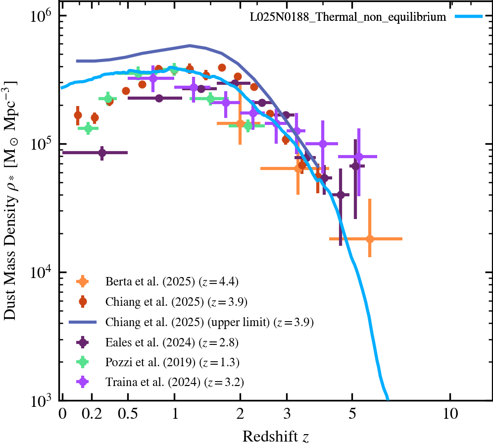
Dust Mass Density Evolution
Evolution of the dust mass density plotted directly from the statistics.txt file produced by SWIFT.
Dust Grain Size Data Comparison
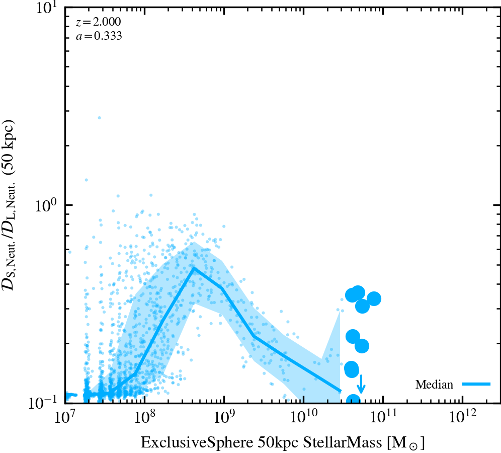
Stellar mass vs Small-to-Large Ratio
The dust mass ratio of small to large grains in all gas aggregated over a 50kpc radius aperture in galaxies. Compared to values derived from observation by Relano et al 2020.
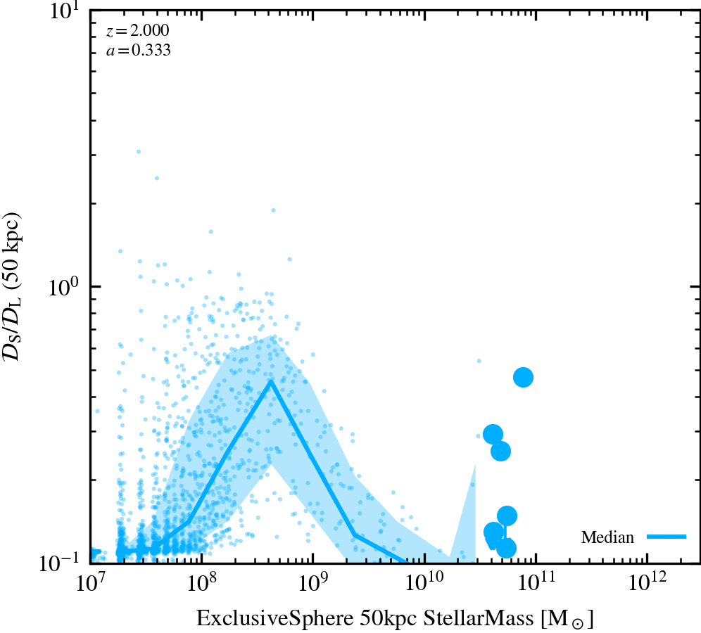
Stellar mass vs Small-to-Large Ratio (H2 only)
The dust mass ratio of small to large grains in all gas aggregated over a 50kpc radius aperture in galaxies. Compared to values derived from observation by Relano et al 2020.
Dust Mass Data Comparison
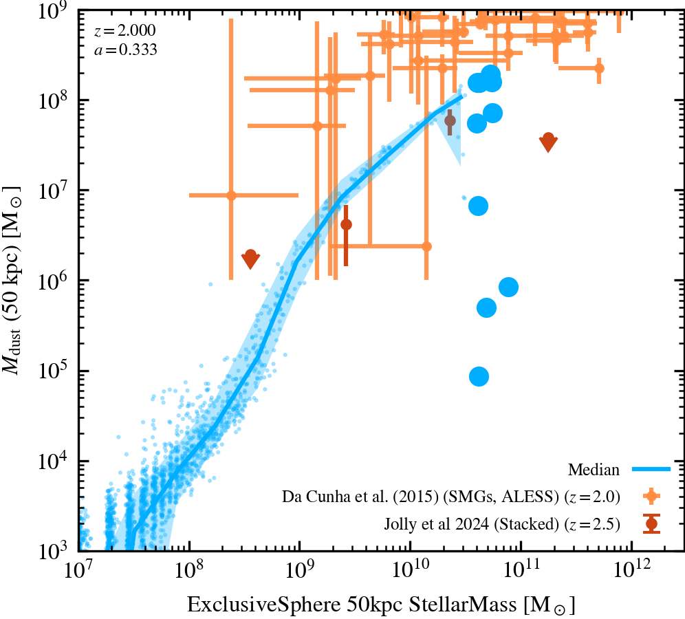
Stellar mass vs Dust Mass
Gas-phase dust mass as a function of stellar mass, high redshift data individual galaxies from ALESS ALMA SMG survey (Da Cunha et al 2015). Data redshifts are photometric.
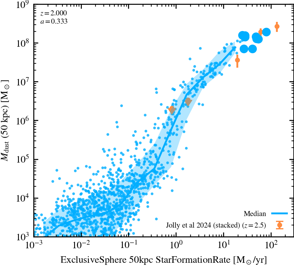
Star formation rate vs Dust Mass
Gas-phase dust mass as a function of SFR, comparing to local Dustpedia galaxies with properties derived using the CIGALE SED fitting code (Bianchi et al 2018)
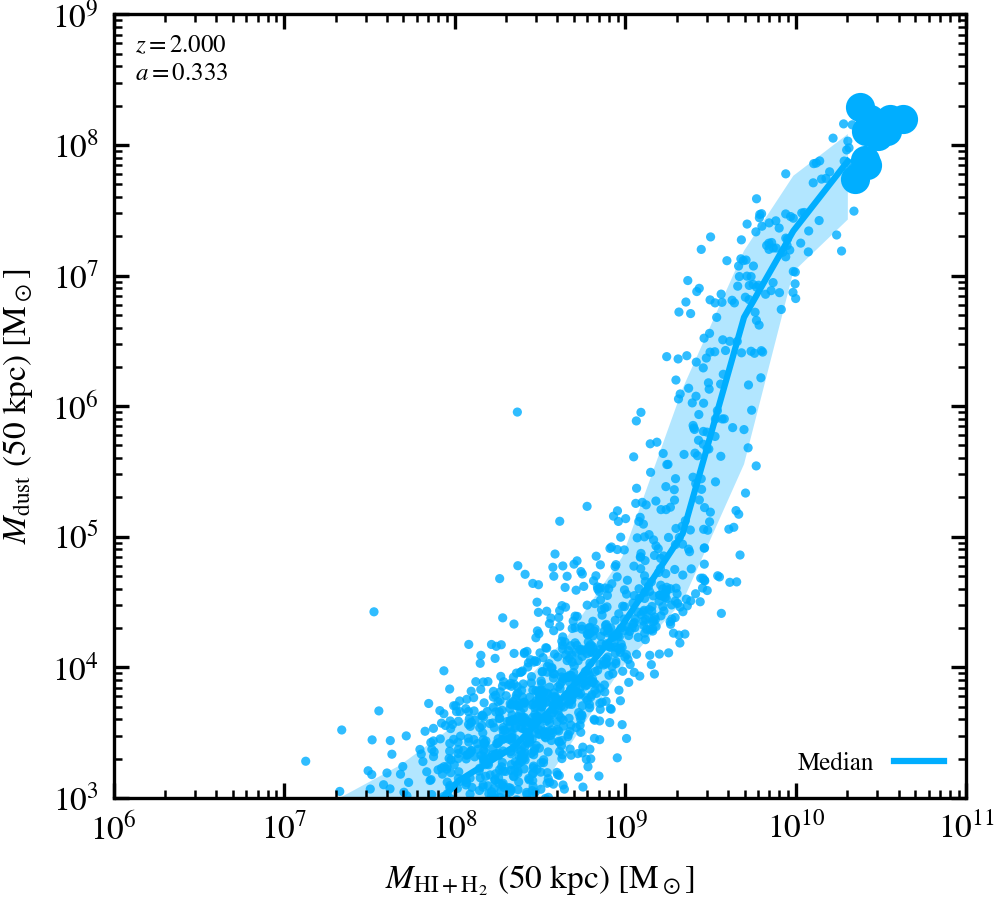
Neutral Gas Mass vs Dust Mass
Gas-phase dust mass as a function of SFR, comparing to local Dustpedia galaxies with properties derived using the CIGALE SED fitting code (Bianchi et al 2018)
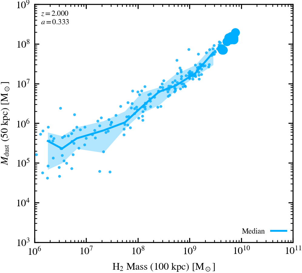
Molecular Gas Mass vs Dust Mass
Gas-phase dust mass as a function of SFR, comparing to local Dustpedia galaxies with properties derived using the CIGALE SED fitting code (Bianchi et al 2018)
Dust Mass Functions
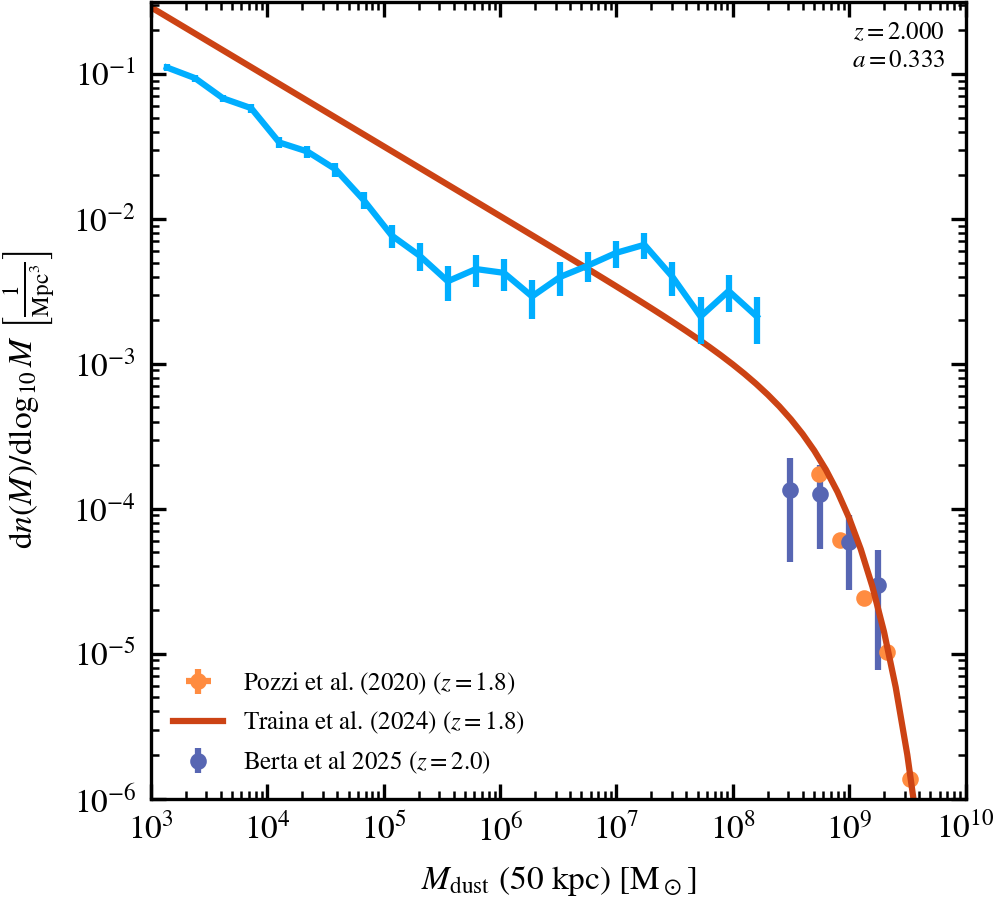
Dust Mass Function
50 kpc aperture Galaxy Dust Mass Function, showing all galaxies with a fixed bin-width of 0.2 dex.
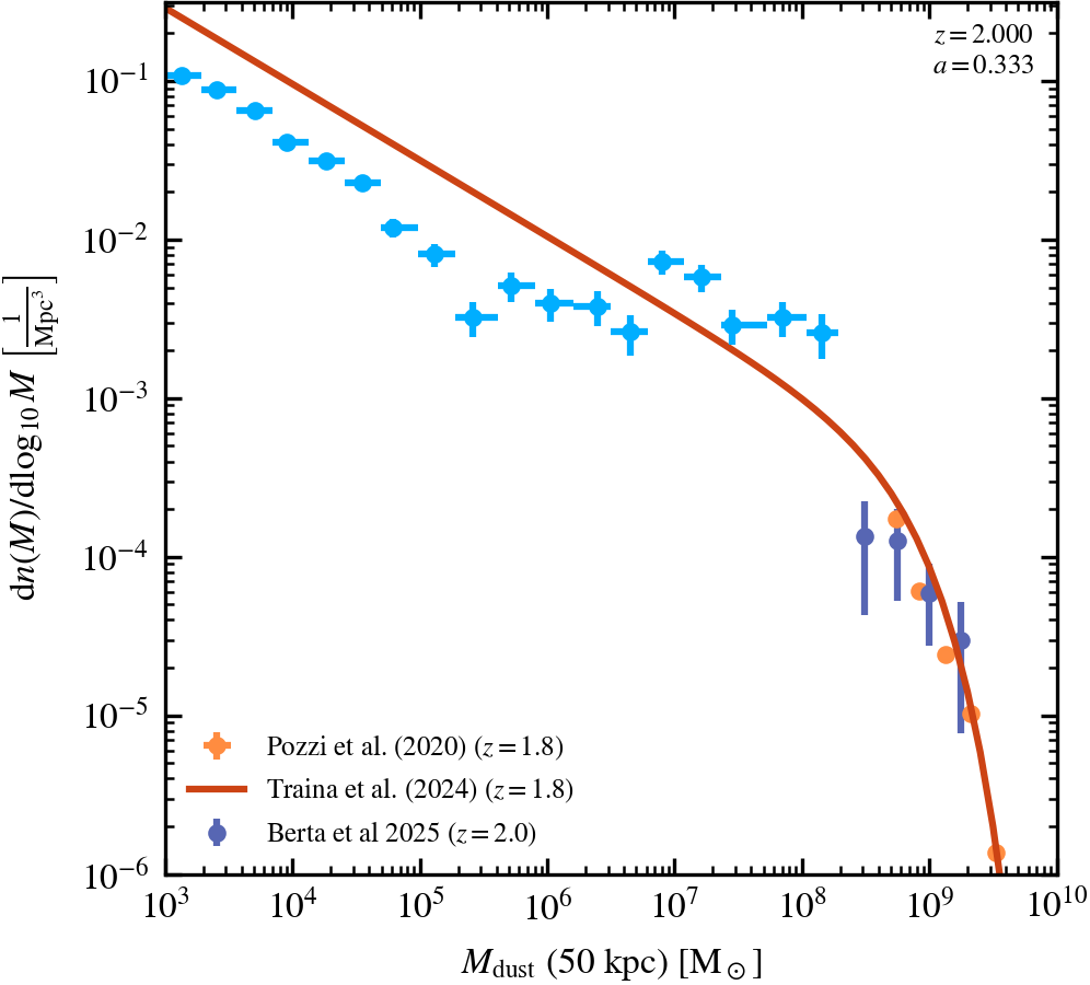
Dust Mass Function
50 kpc aperture Galaxy Dust Mass Function, showing all galaxies with an adaptive bin-width.
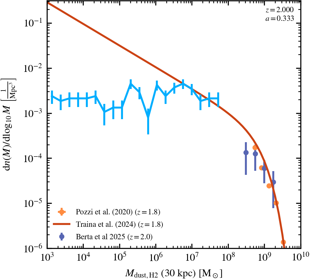
Molecular Dust Mass Function
30 kpc aperture Galaxy Dust Mass Function, showing all galaxies with a fixed bin-width of 0.2 dex.
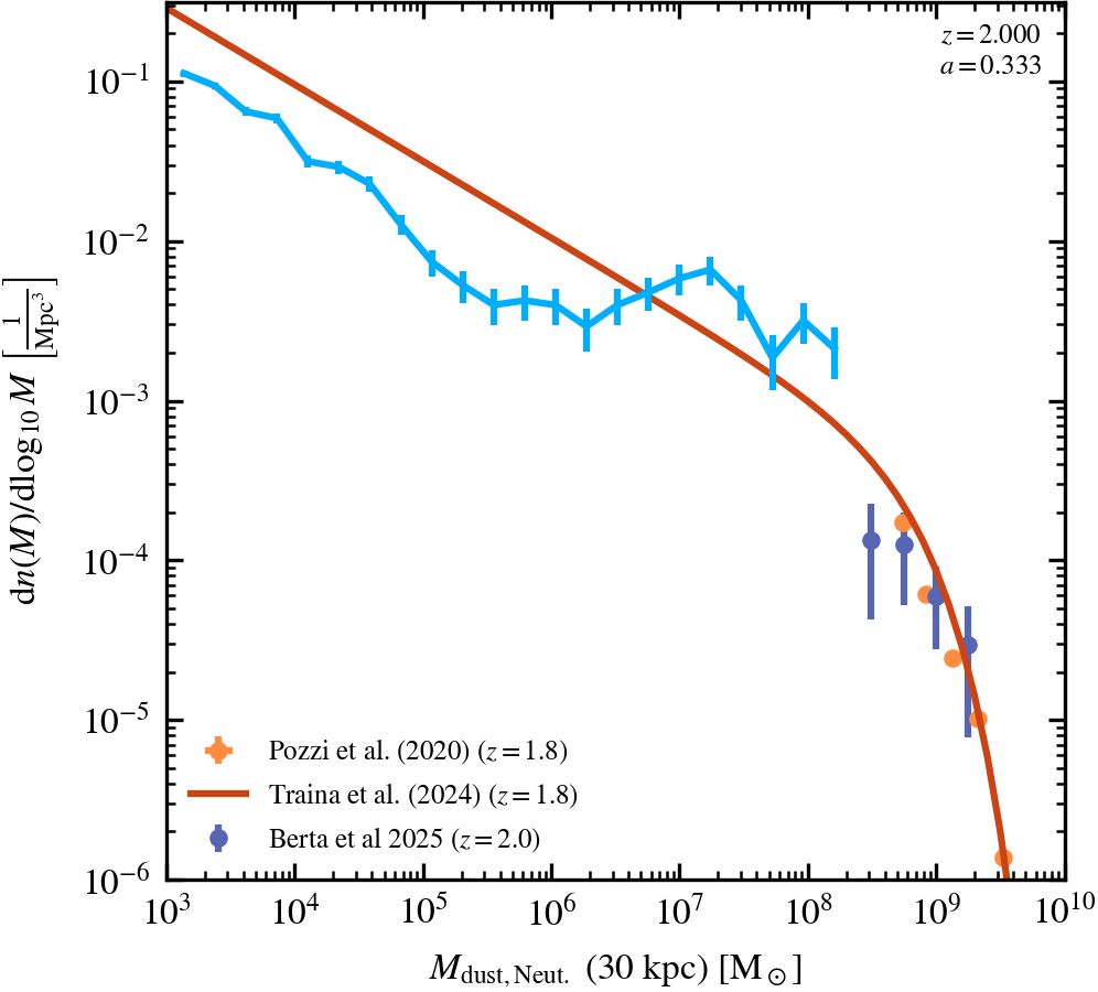
Neutral Dust Mass Function
30 kpc aperture Galaxy Dust Mass Function, showing all galaxies with a fixed bin-width of 0.2 dex.
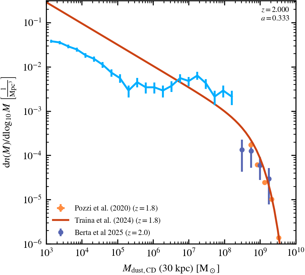
Cold Dense Dust Mass Function
30 kpc aperture Galaxy Dust Mass Function, showing all galaxies with a fixed bin-width of 0.2 dex.
Dust Scaling Relations (ISM Selection)
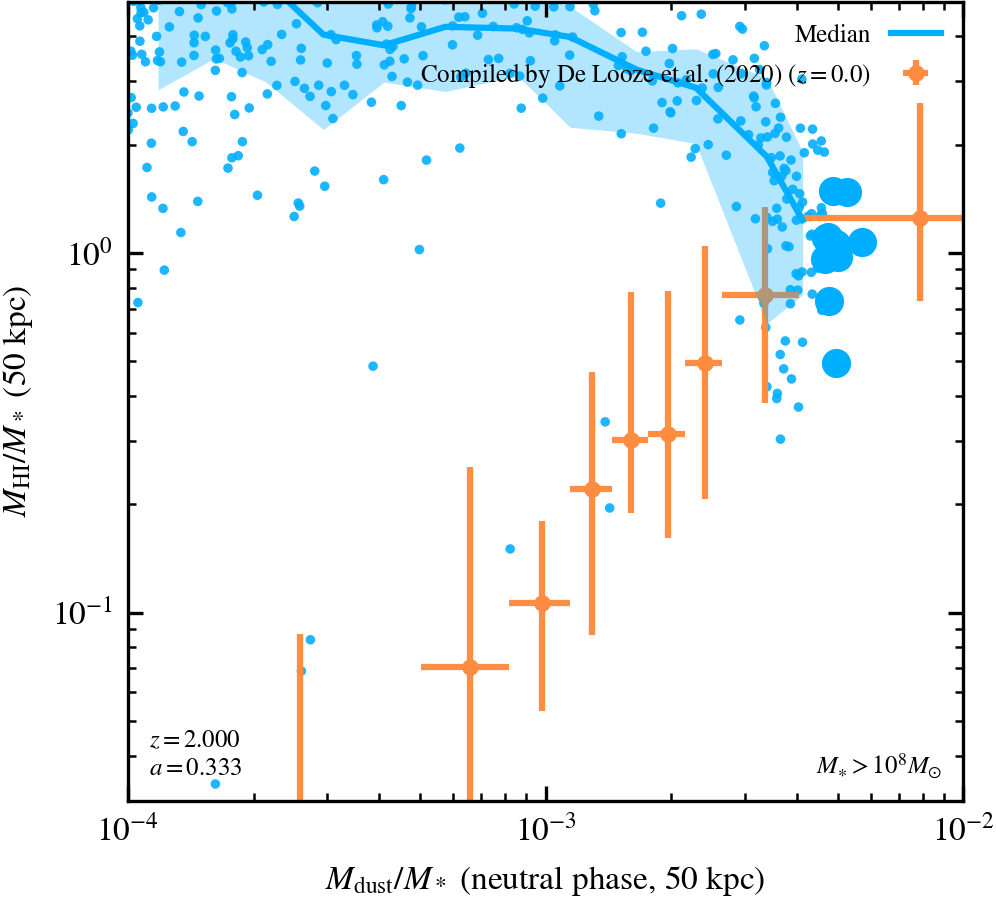
HI-to-stellar mass ratio vs dust-to-stellar mass ratio in neutral gas.
HI to stellar mass ratio as a function of the dust-to-stellar mass ratio in neutral gas measured in 50kpc apertures, and applying a JINGLE-like mass selection.
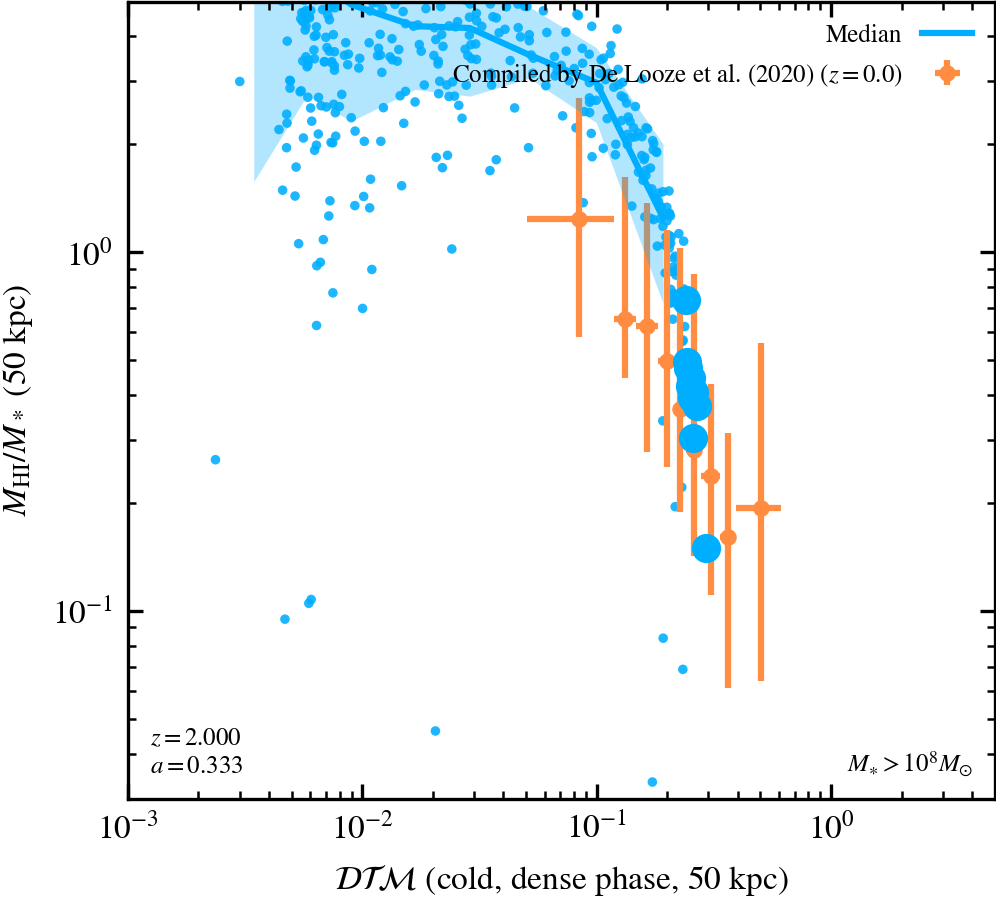
HI-to-stellar mass ratio vs dust-to-metal ratio in cold, dense gas
HI to stellar mass ratio as a function of the dust-to-metal ratio in cold, dense gas ($T < 10^{4.5}\;{\rm K}$, $n_{\rm H} > 0.1 \; {\rm cm^{-3}}$) measured in 50kpc apertures, and applying a JINGLE-like mass selection.
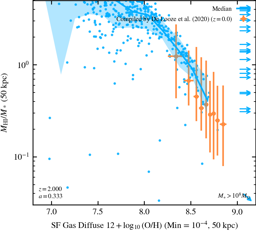
HI-to-stellar mass ratio vs Oxygen abundance
HI to stellar mass ratio as a function of the gas-phase Oxygen abundance measured in 50 kpc apertures, and applying a JINGLE-like mass selection.
Feedback Densities
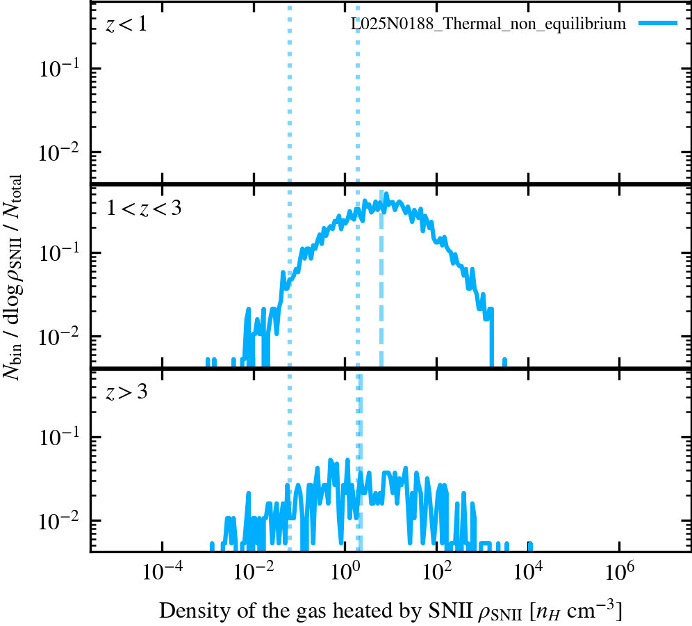
Density of the gas heated by SNII
Distributions of the gas densities recorded when the gas was last heated by SNII, split by redshift. The y axis shows the number of SNII-heated gas particles per bin divided by the bin width and by the total of SNII-heated gas particles. The dashed vertical lines show the median SNII gas-densities, while the dotted lines indicade the critical density from C. Dalla Vecchia & J. Schaye (2012) for SN min and max heating temperatures with $f_t=10$. Star particles are not included.
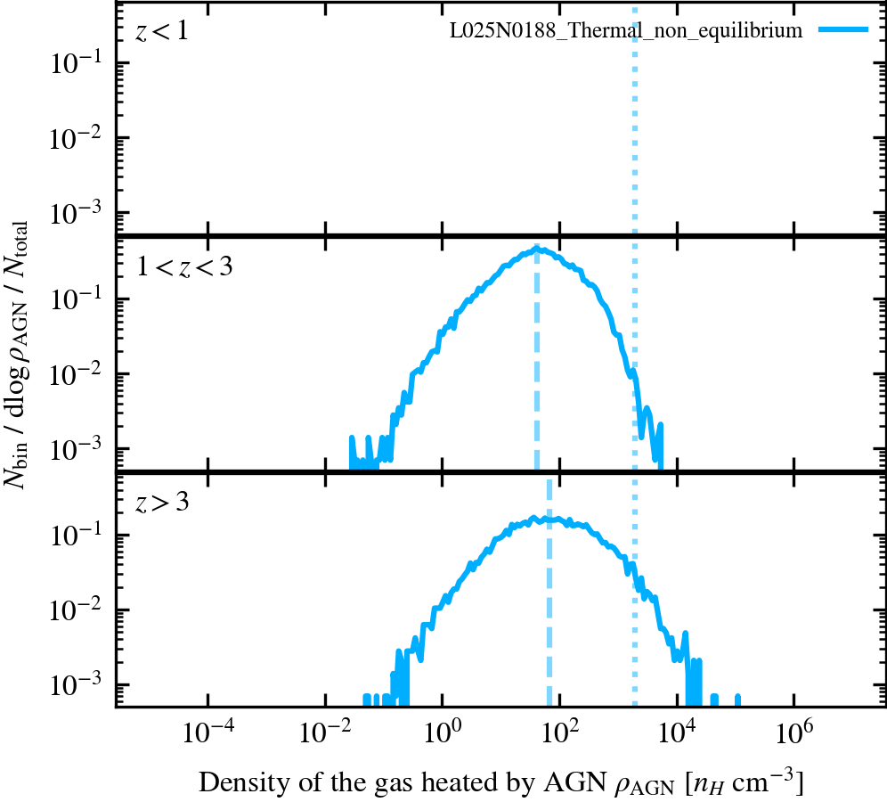
Density of the gas heated by AGN
Distributions of the gas densities recorded when the gas was last heated by AGN, split by redshift. The y axis shows the number of AGN-heated gas particles per bin divided by the bin width and by the total of AGN-heated gas particles. The dashed vertical lines show the median AGN gas-densities, while the dotted lines indicade the critical density from C. Dalla Vecchia & J. Schaye (2012) for AGN heating temperature with $f_t=10$. Star particles not included.
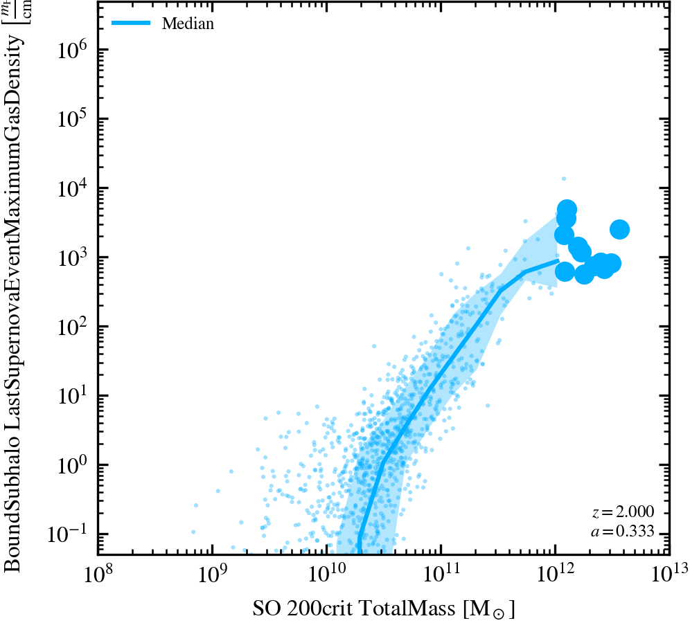
Maximal SNII thermal feedback Density-Halo Mass relation
Includes all haloes, including subhaloes.
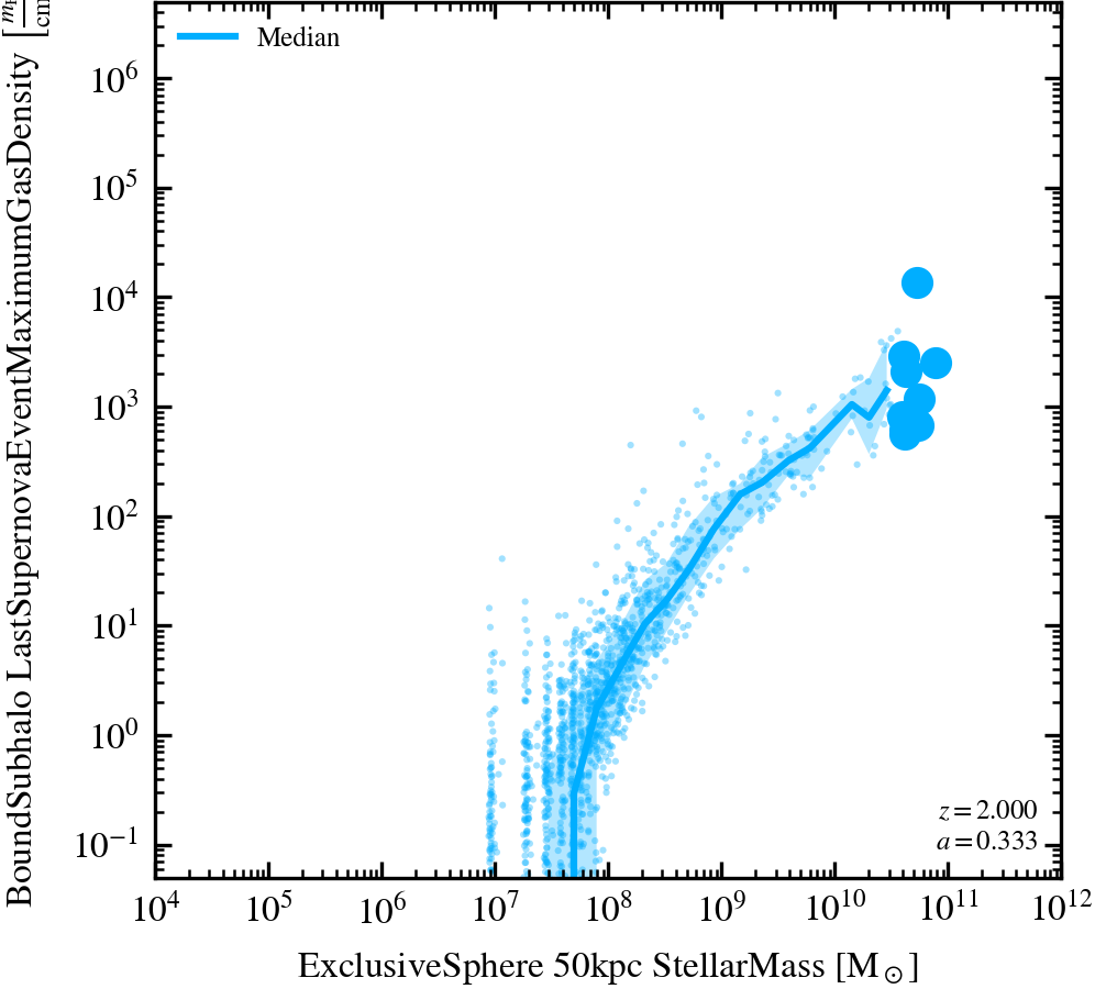
Maximal SNII thermal feedback Density-Stellar Mass relation
Includes all haloes, including subhaloes.
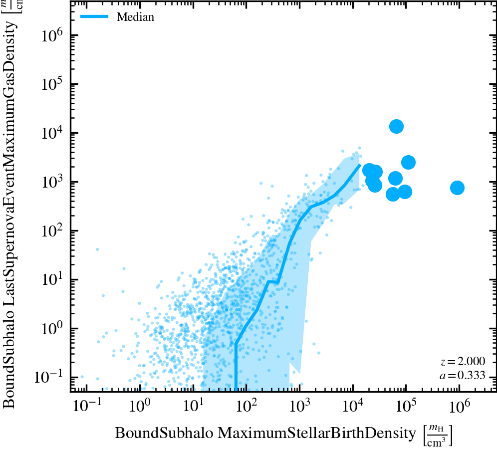
Maximal SNII thermal feedback Density-Maximal Stellar Birth Density relation
Includes all haloes, including subhaloes.
Feedback kick velocities
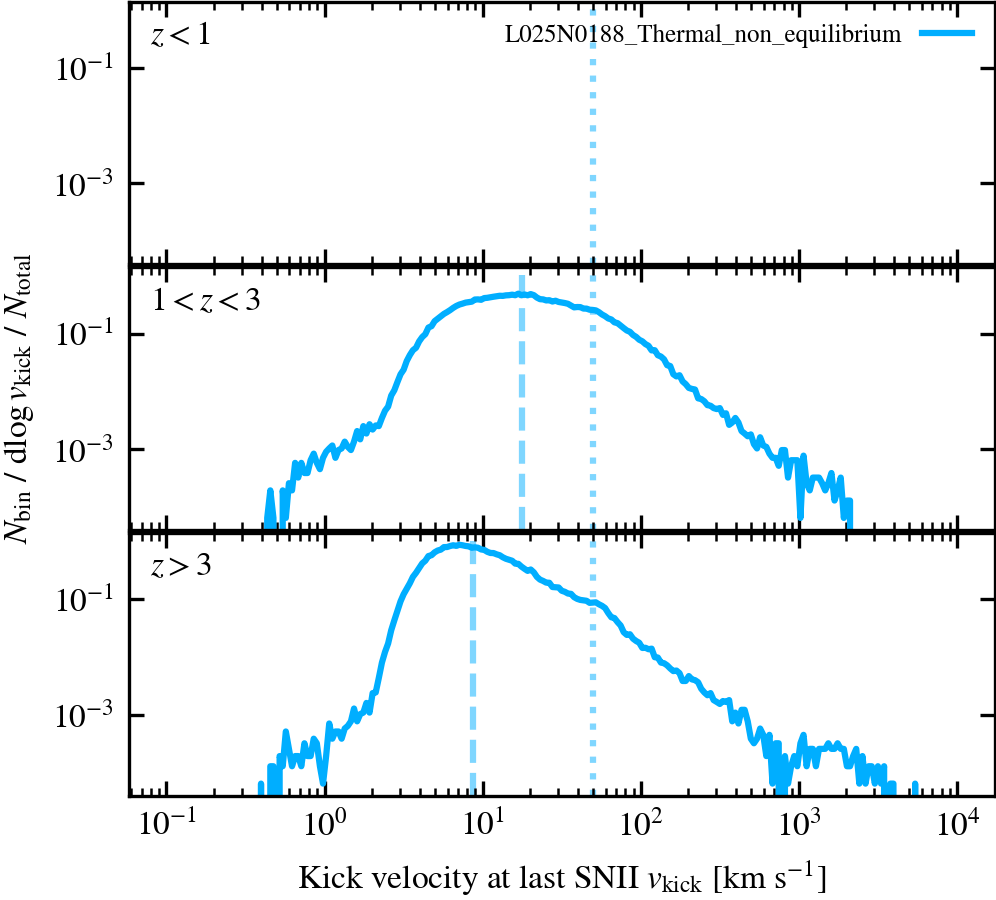
Kick velocity distribution at last SNII
Distributions of SNII kick velocities experienced by the gas recorded when the gas was last kicked by SNII, split by redshift. The y axis shows the number of SNII-kicked gas particles per bin divided by the bin width and by the total of SNII-kicked gas particles. The dashed vertical lines show the median kick velocitites, while the dotted lines indicade the target kick velocity. Star particles are not included.
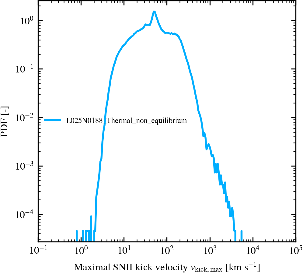
Maximal SNII kick velocity
Maximal SNII kick velocities by experienced by particles in SNII kinetic feedback throughout the entire simulation.
Gas Mass Function
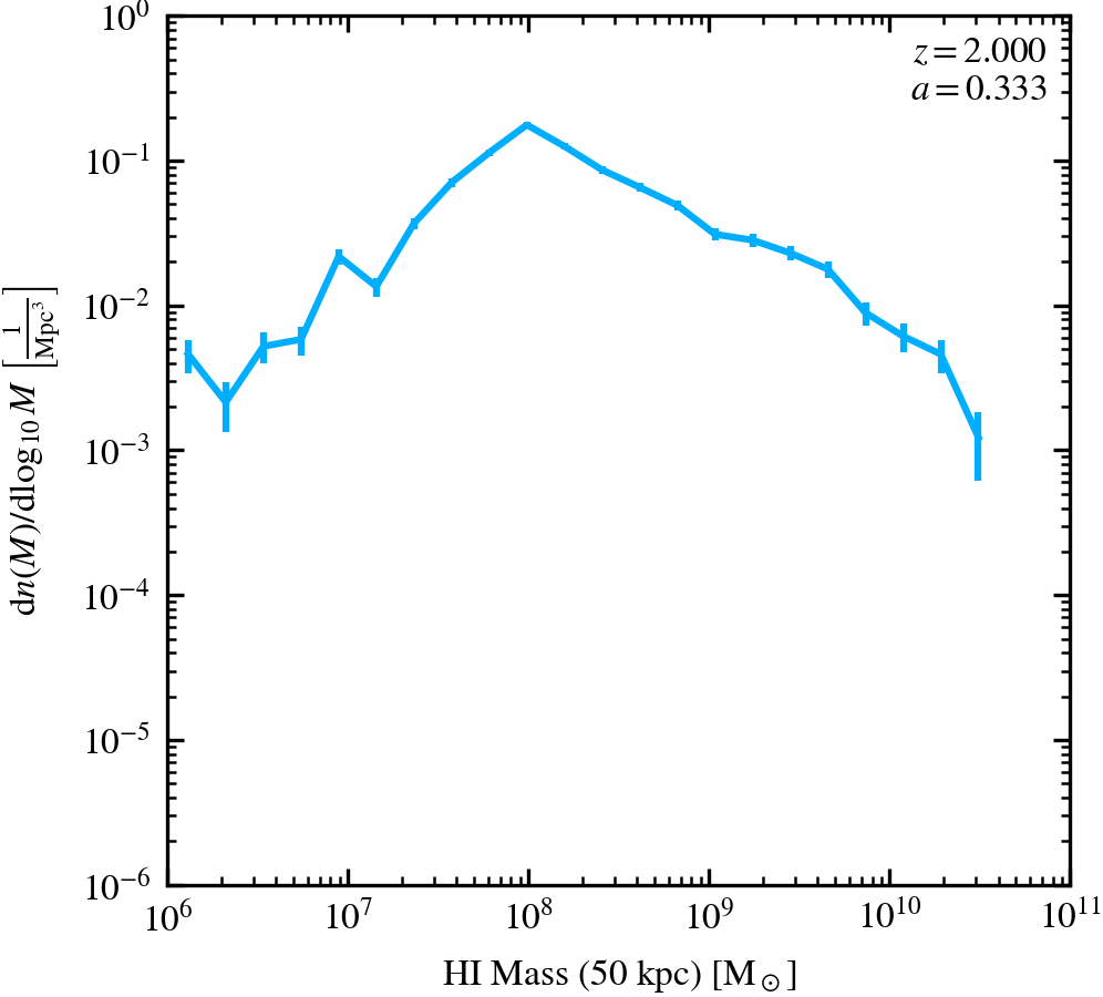
HI Mass Function
HIMF, showing all galaxies with a fixed bin-width of 0.2 dex (HI masses 50 kpc).
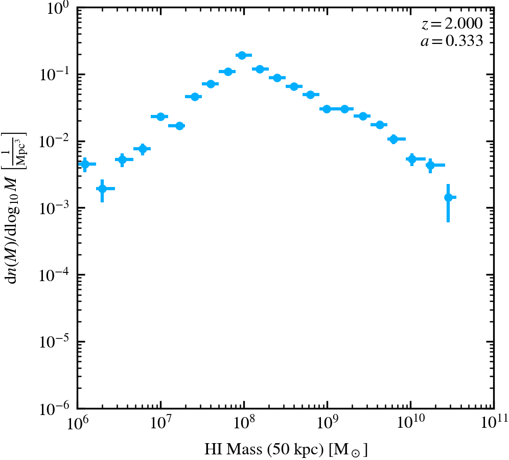
HI Mass Function
HIMF, showing all galaxies with an adaptive bin-width (HI masses 50 kpc).
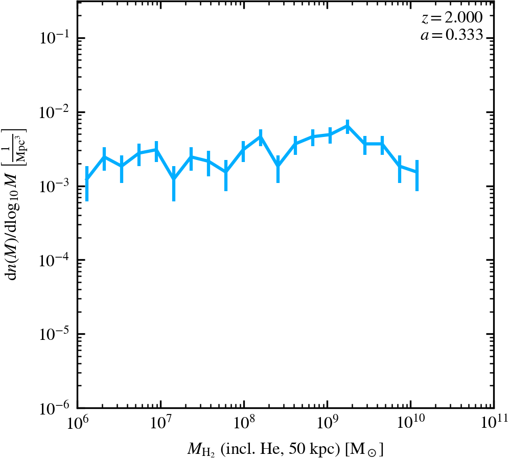
H$_2$ Mass Function
H$_2$ MF, showing all galaxies with a fixed bin-width of 0.2 dex. H$_2$ mass corrected for Helium (uses H$_2$ masses in 50 kpc apertures)
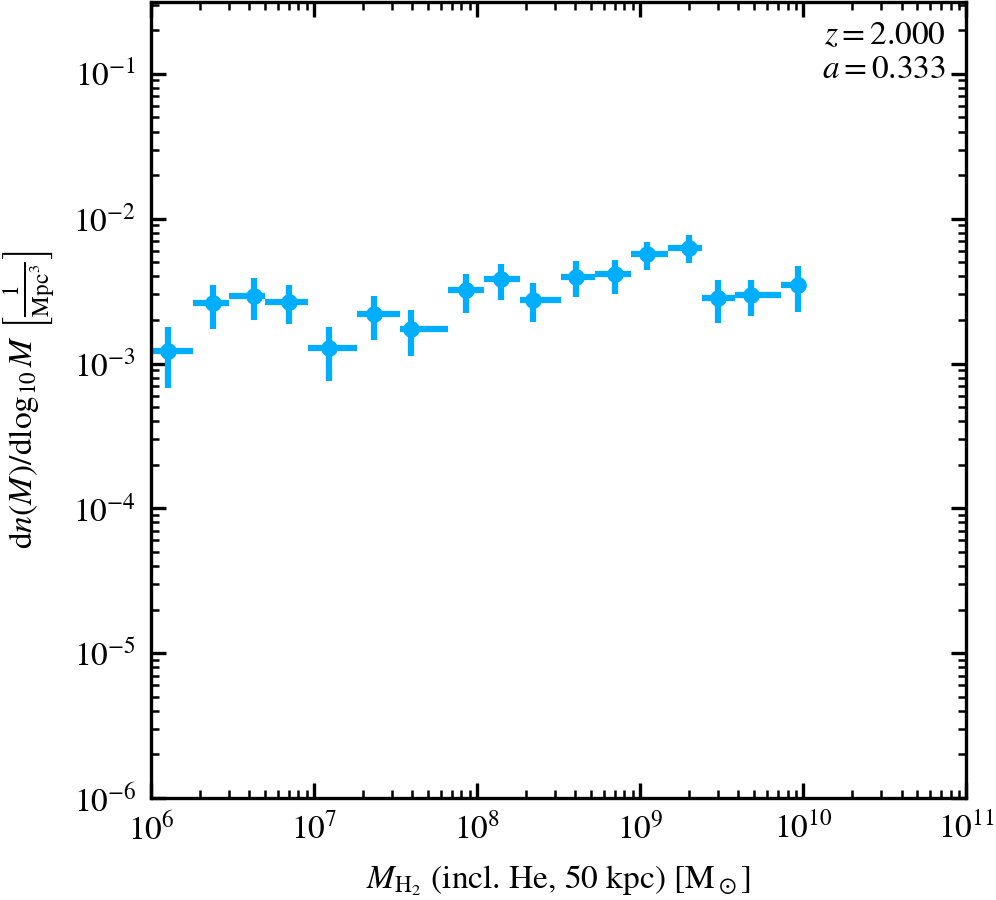
H$_2$ Mass Function
H$_2$ MF, showing all galaxies with an adaptive bin-width. H$_2$ mass corrected for Helium (uses H$_2$ masses in 50 kpc apertures)
Gas Metallicity
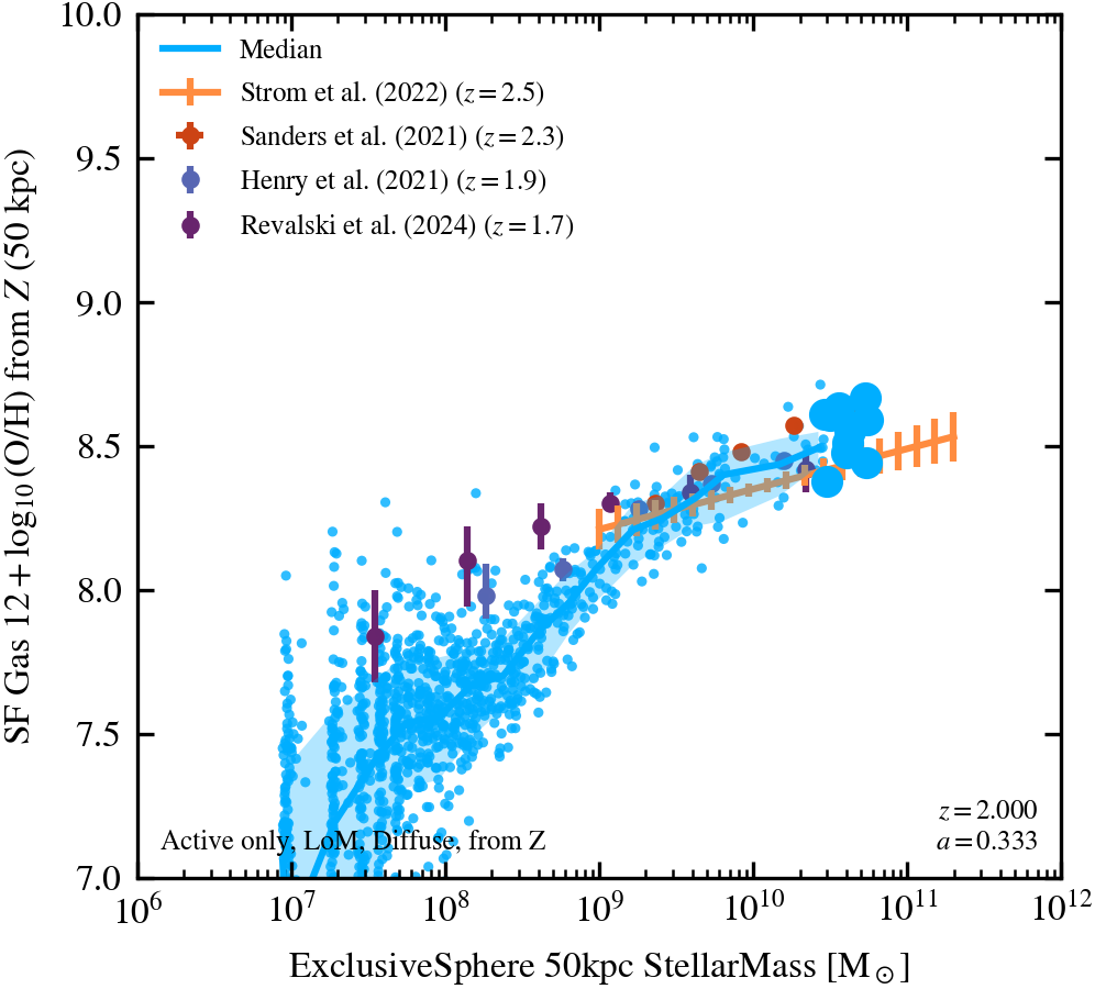
Stellar mass - Gas diffuse metallicity relation (log-of-mean, from Z, 50 kpc aperture)
Only shown for star forming galaxies. Computed as the average mass-weighted metal mass fraction (converted to 12 + $\log_{10}$ O/H by assuming solar abundance patterns) of cold, dense gas ($T < 10^{4.5}\;{\rm K}$, $n_{\rm H} > 0.1 \; {\rm cm^{-3}}$). No minimum metallicity is imposed. All haloes are plotted, including subhaloes. This uses depleted gas metallicity, i.e. it does not include metals that are present in dust.
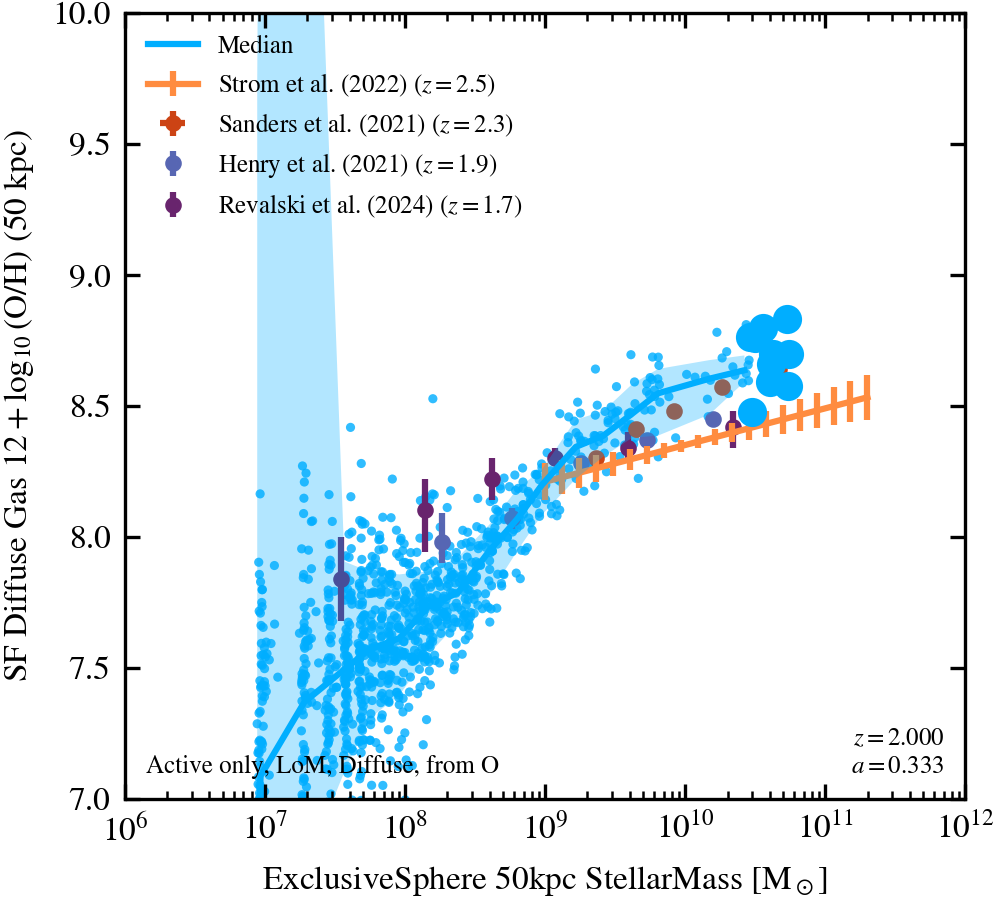
Stellar mass - Gas diffuse metallicity relation (log-of-mean, 50 kpc aperture)
Only shown for star forming galaxies. Represented by 12 + $\log_{10}$ O/H (where O/H is linearly averaged for diffuse O) of the cold, dense gas ($T < 10^{4.5}\;{\rm K}$, $n_{\rm H} > 0.1 \; {\rm cm^{-3}}$). No minimum metallicity is imposed. All haloes are plotted, including subhaloes. This uses depleted gas metallicity, i.e. it does not include metals that are present in dust.
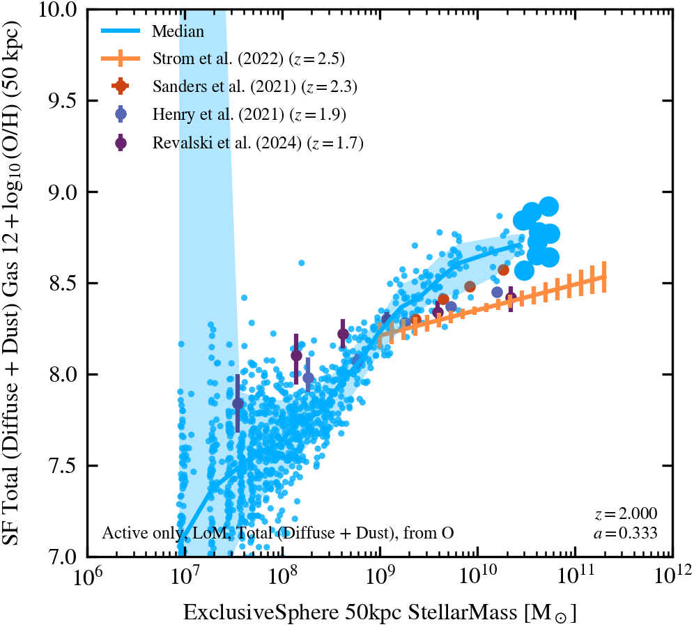
Stellar mass - Gas (Diffuse + Dust) metallicity relation (log-of-mean, 50 kpc aperture)
Only shown for star forming galaxies. Represented by 12 + $\log_{10}$ O/H (where O/H is linearly averaged for total O) of the cold, dense gas ($T < 10^{4.5}\;{\rm K}$, $n_{\rm H} > 0.1 \; {\rm cm^{-3}}$). No minimum metallicity is imposed. All haloes are plotted, including subhaloes. This uses undepleted gas metallicity, i.e. it includes metals that are present in dust.
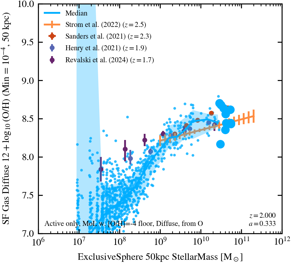
Stellar mass - Gas diffuse metallicity relation (mean-of-log, 50 kpc aperture)
Only shown for star forming galaxies. Represented by 12 + $\log_{10}$ O/H (where $\log_{10}$ O/H is averaged between gas particles with a [O/H]=-4 floor and diffuse O) of the cold, dense gas ($T < 10^{4.5}\;{\rm K}$, $n_{\rm H} > 0.1 \; {\rm cm^{-3}}$). All haloes are plotted, including subhaloes. This uses depleted gas metallicity, i.e. it does not include metals that are present in dust.
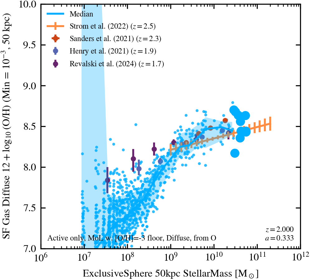
Stellar mass - Gas diffuse metallicity relation (mean-of-log, 50 kpc aperture)
Only shown for star forming galaxies. Represented by 12 + $\log_{10}$ O/H (where $\log_{10}$ O/H is averaged between gas particles with a [O/H]=-3 floor for diffuse O) of the cold, dense gas ($T < 10^{4.5}\;{\rm K}$, $n_{\rm H} > 0.1 \; {\rm cm^{-3}}$). All haloes are plotted, including subhaloes. This uses depleted gas metallicity, i.e. it does not include metals that are present in dust.
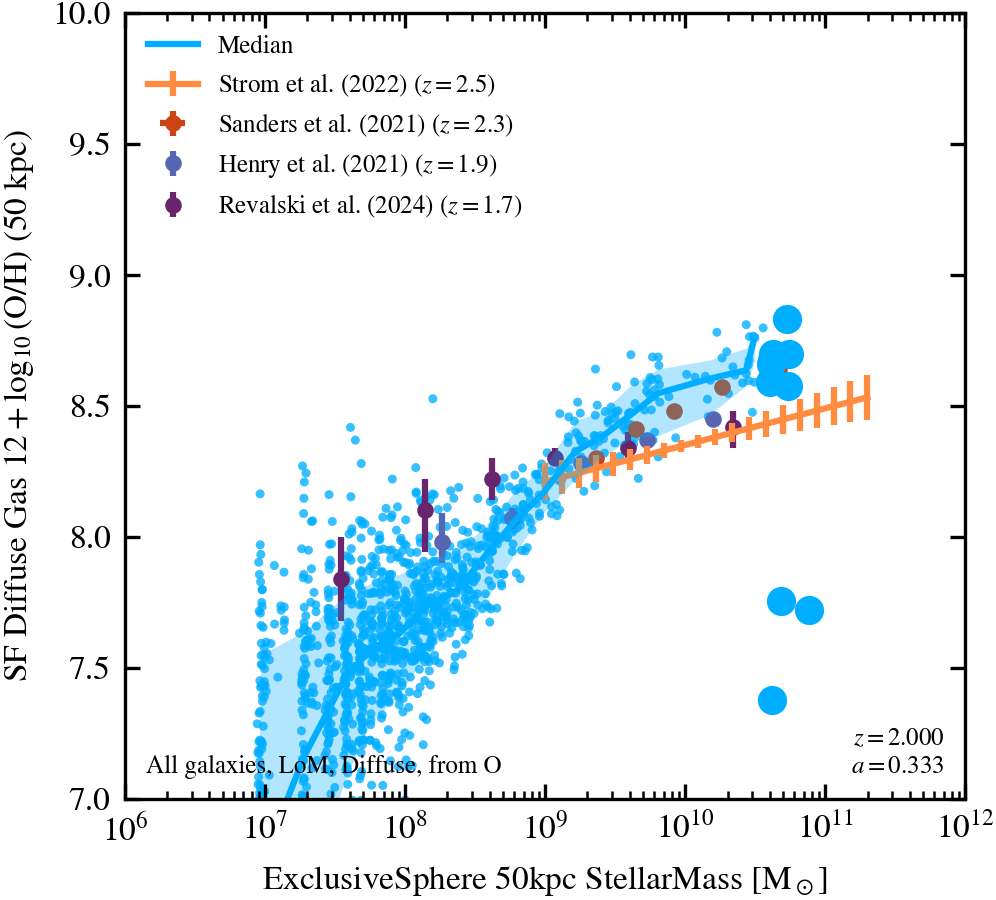
Stellar mass - Gas diffuse metallicity relation (log-of-mean, 50 kpc aperture)
Only shown for galaxies with cold, dense gas. Represented by 12 + $\log_{10}$ O/H (where O/H is linearly averaged for diffuse O) of the cold, dense gas ($T < 10^{4.5}\;{\rm K}$, $n_{\rm H} > 0.1 \; {\rm cm^{-3}}$). No minimum metallicity is imposed. All haloes are plotted, including subhaloes. This uses depleted gas metallicity, i.e. it does not include metals that are present in dust.
Halo Mass Function
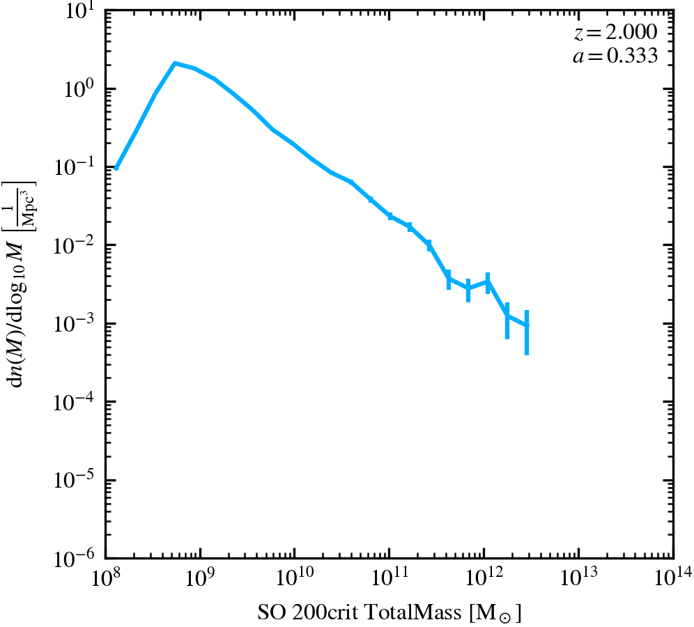
Halo Mass Function ($M_{200, crit}$)
Halo masses are masses within the over-density radius enclosing 200x the critical density, using 0.2 dex fixed bin-widths (centrals only).
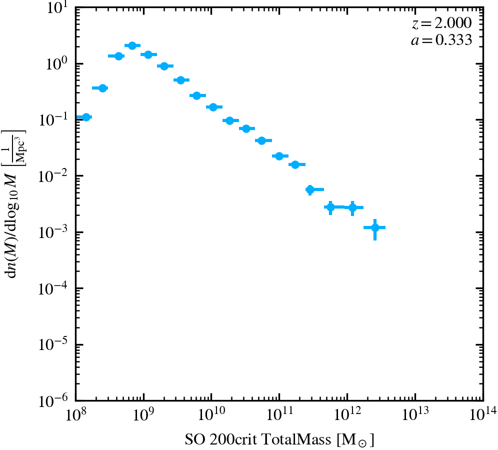
Halo Mass Function ($M_{200, crit}$)
Halo masses are masses within the over-density radius enclosing 200x the critical density, using adaptive binning (centrals only).
Histograms
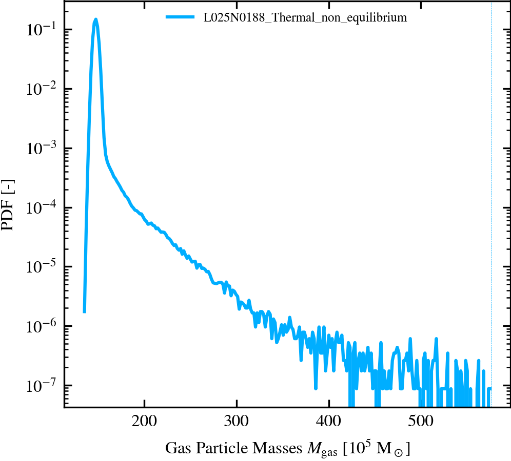
Gas Particle Masses
Gas Particle Masses with the threshold for splitting indicated by the vertical dashed line.
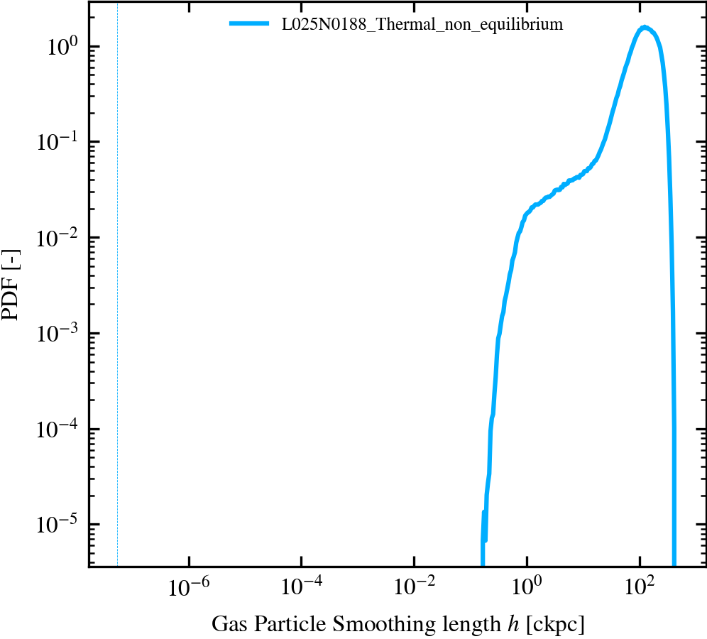
Gas Particle Smoothing Lengths
Gas Particle Comoving Smoothing Lengths with the minimal smoothing length indicated by the vertical dashed line.
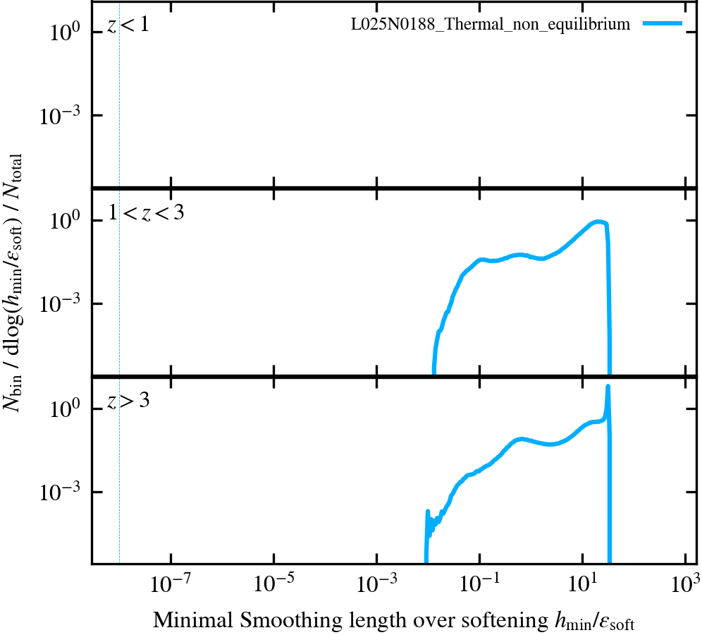
Gas Particle Minimal Smoothing Lengths
Gas Particle Comoving Minimal Smoothing Lengths reached during the simulation, split by redshifts at which these minimal smoothing lengths were reached and normalised by the gravitational softening length (at the corresponding redshift). The minimal allowed ratio between smoothing length and gravitational softening length is indicated by the vertical dashed line. The normalisation by the softening includes the factor of 3 to convert from the Plummer-equivalent softening length, which is specified in the parameter file. The normalisation also accounts for the factor of $\gamma_{\rm kernel} \approx 2$, which relates the smoothing length to the extent of an SPH kernel.
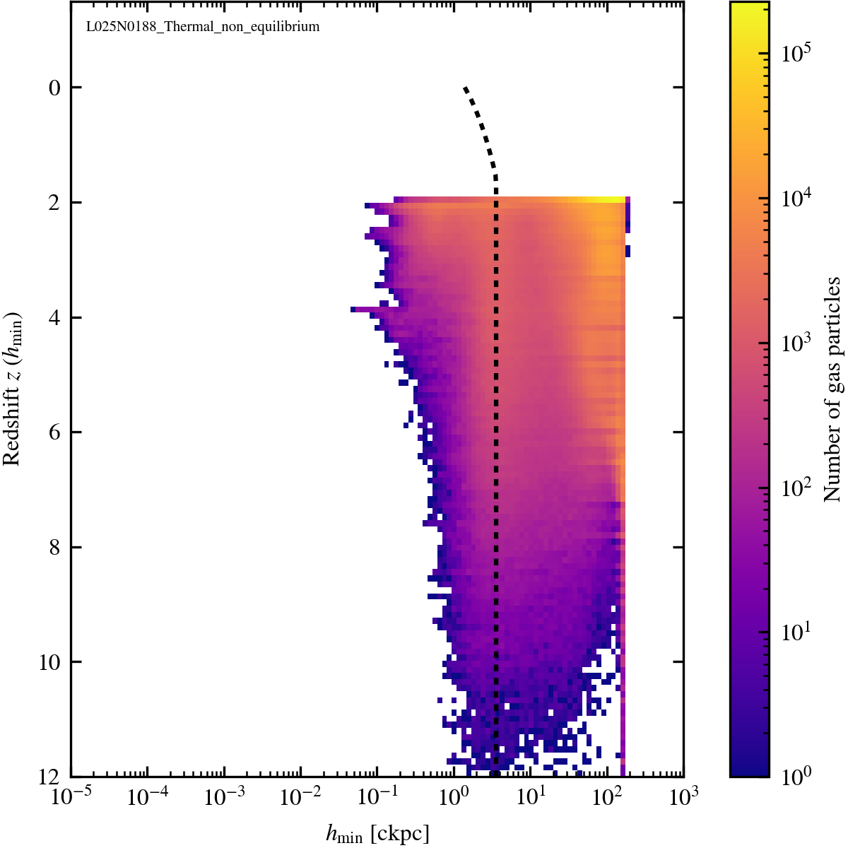
Gas Particle Minimal Smoothing Lengths vs. Redshift
Gas Particle Comoving Minimal Smoothing Lengths versus Redshifts at which these minimal smoothing lengths were reached. The black dashed and black dotted curves indicate, respectively, the minimum allowed smoothing length and gravitational softening length at a given redshift.
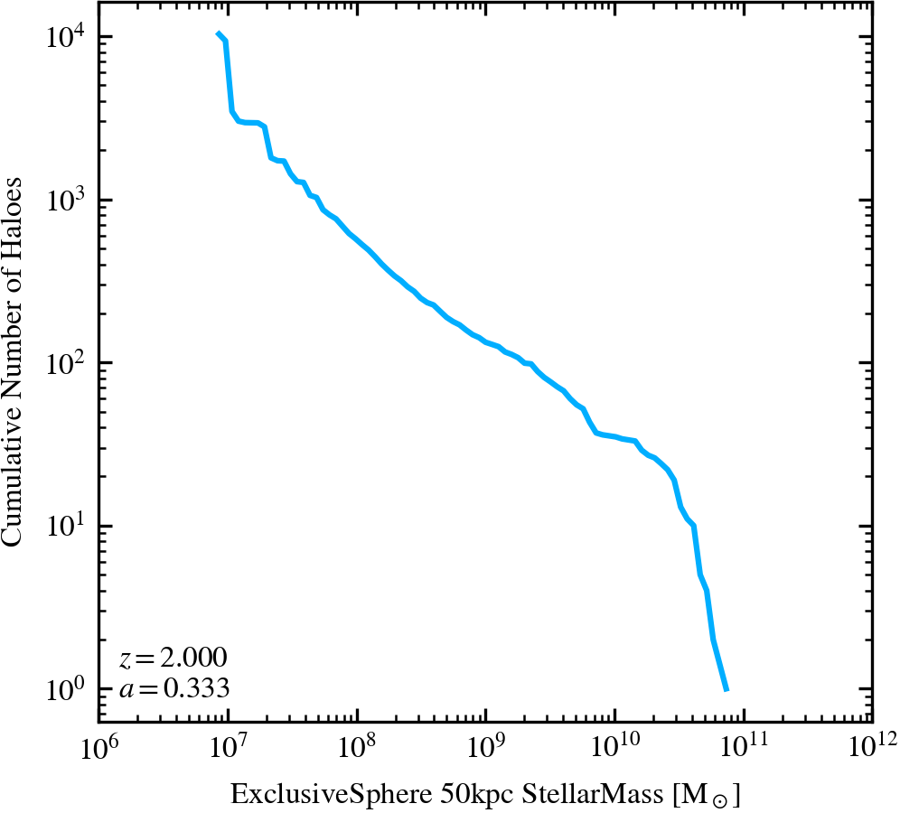
Stellar Mass Histogram (50 kpc aperture)
Cumulative histogram of stellar masses using the same bins as the mass function.
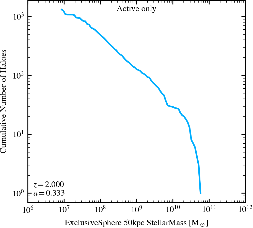
Stellar Mass Histogram (50 kpc aperture, active)
Only for active galaxies.
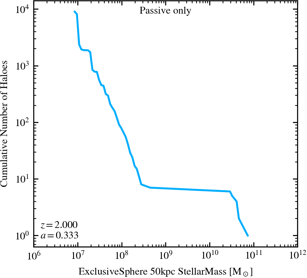
Stellar Mass Histogram (50 kpc aperture, passive)
Only for passive galaxies.
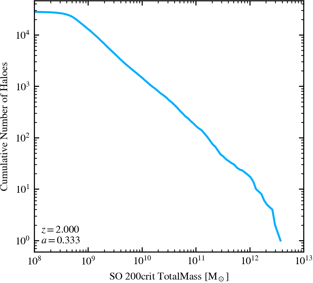
Halo Mass Histogram (\(M_{200, crit}\))
All halo masses (200 crit).
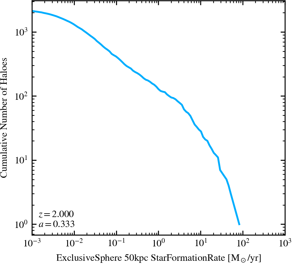
Star Formation Rate Histogram (50 kpc aperture)
Cumulative histogram of star formation rates using the same bins as the star formation rates function.
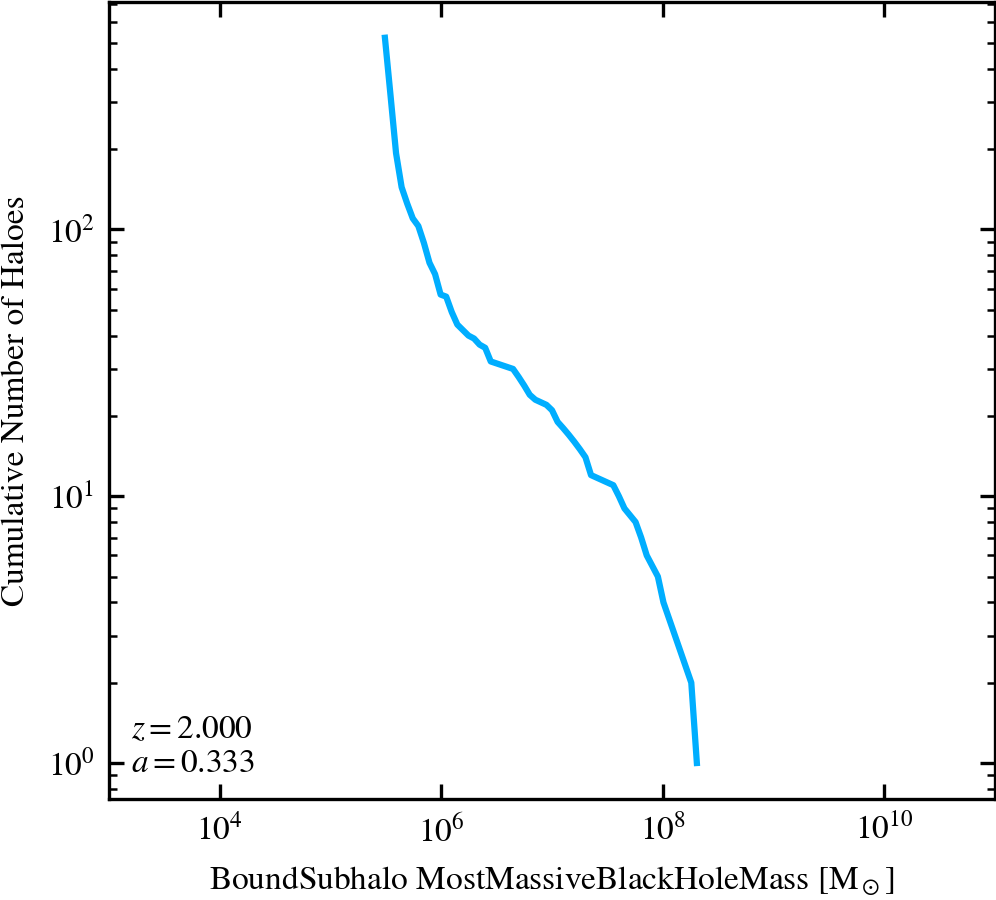
Black Hole Mass Histogram (Max, subgrid)
Uses the same bins as in the black holes section.
Hydrogen Phase Density-Temperature
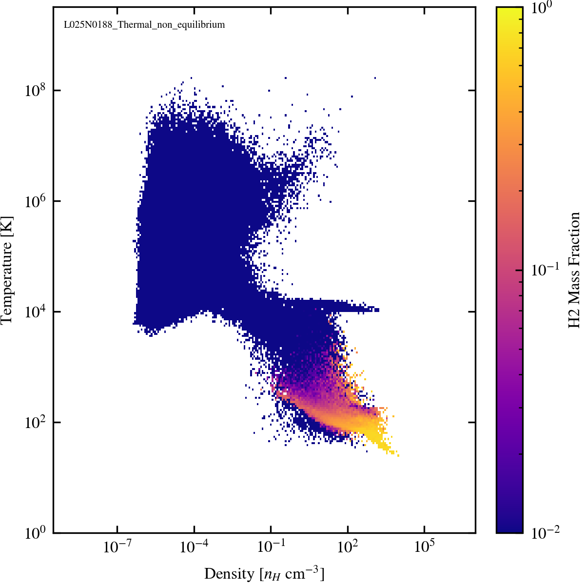
H$_2$
Density-temperature diagram shaded by H$_2$ mass fraction. The fraction is computed as the H$_2$ mass contained in each cell over the mass of gas in that cell.
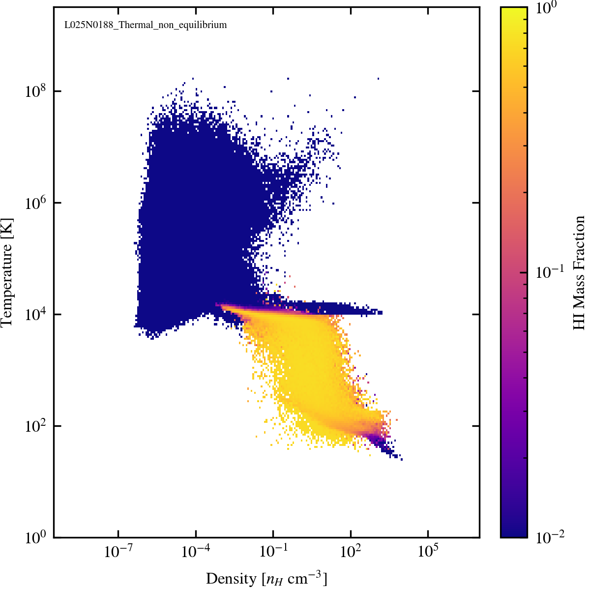
HI
Density-temperature diagram shaded by HI mass fraction. The fraction is computed as the HI mass contained in each cell over the mass of gas in that cell.
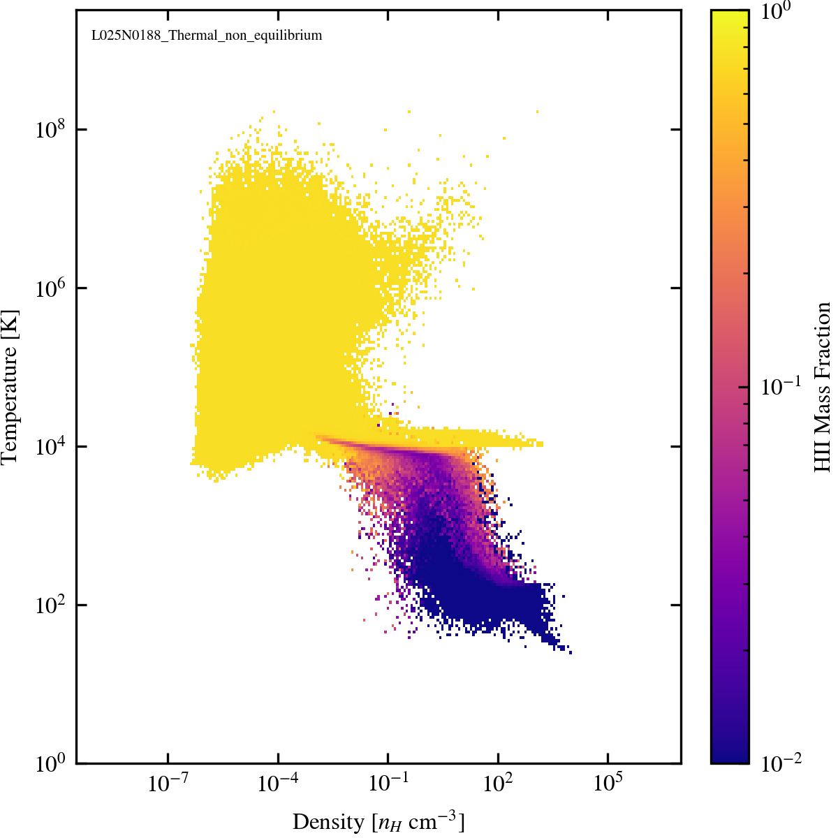
HII
Density-temperature diagram shaded by HII mass fraction. The fraction is computed as the HII mass contained in each cell over the mass of gas in that cell.
Hydrogen Phases
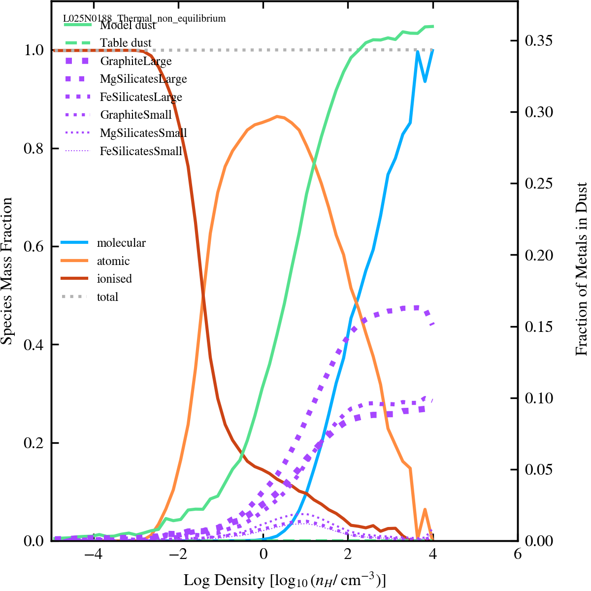
Hydrogen Phase Fractions
Co-plot of species fractions (left y-axis) and the dust-to-metal ratio (right y-axis) as a function opf gas density. If available, solid green line shows explicitly modelled dust-to-metal ratio, while dashed green is interpolated from the Ploeckinger+20 tables.
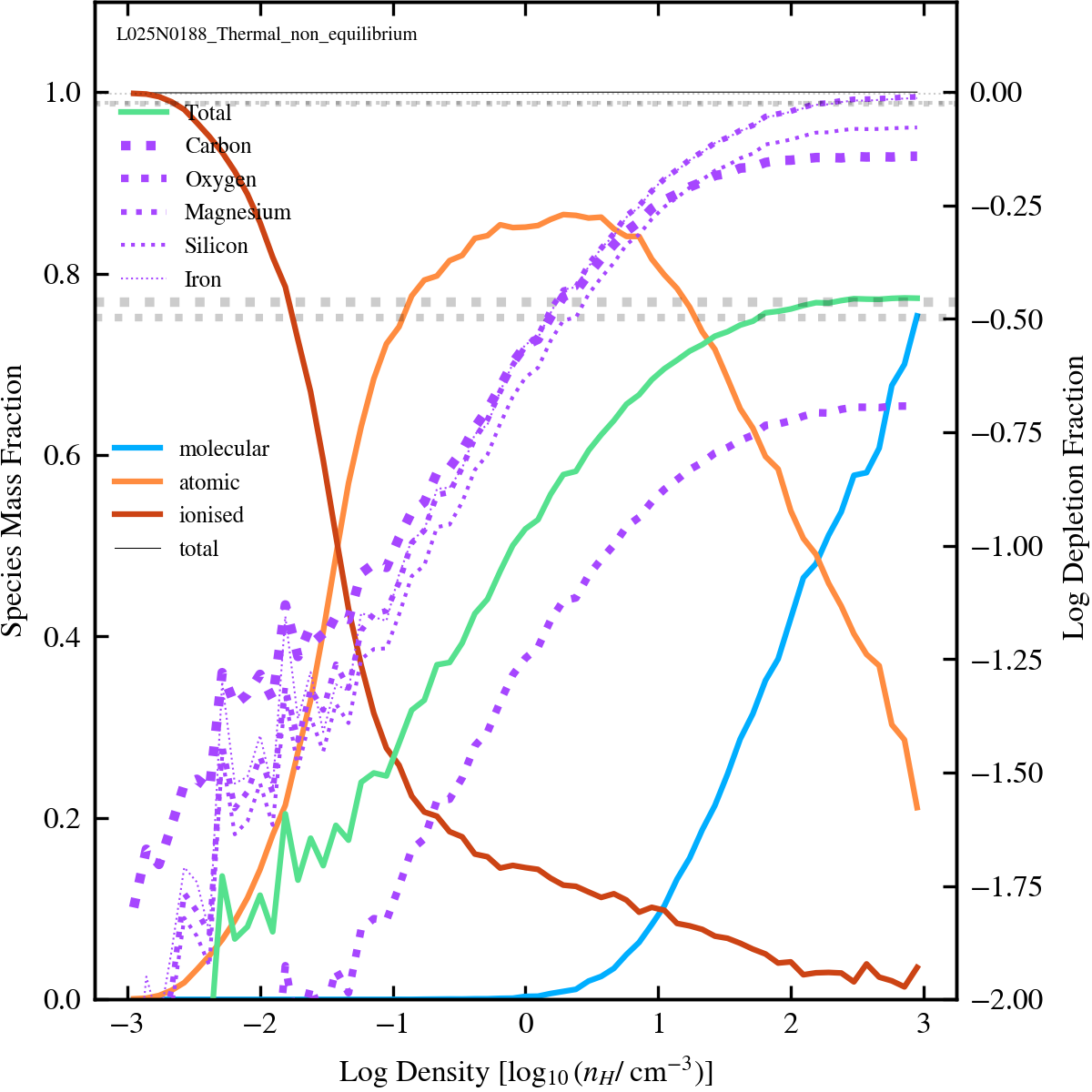
Hydrogen Phase Fractions (Depletion Fraction)
Co-plot of species fractions (left y-axis) and the dust-to-metal ratio (right y-axis) as a function of gas density. If available, solid green line shows explicitly modelled dust-to-metal ratio, while dashed green is interpolated from the Ploeckinger+20 tables.
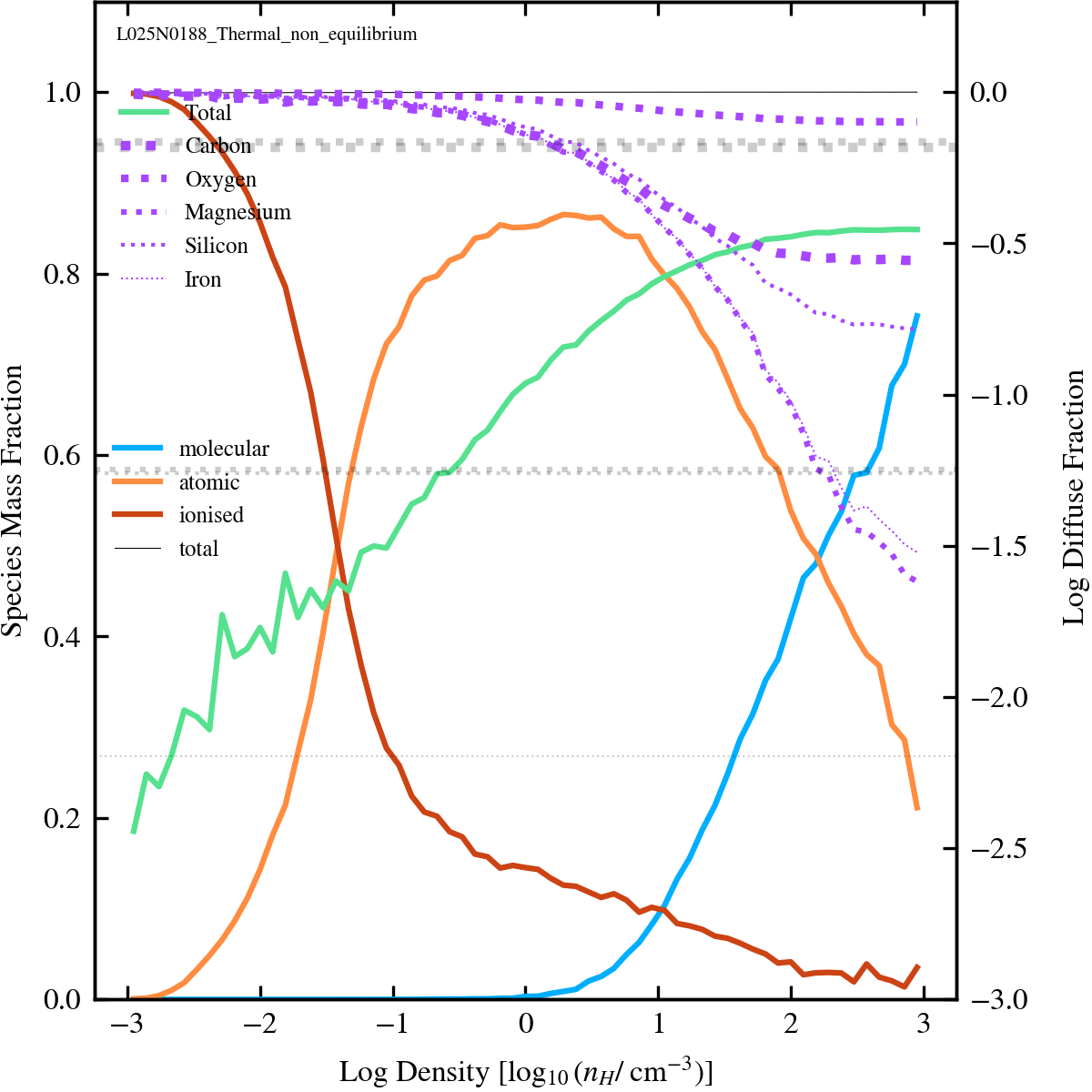
Hydrogen Phase Fractions (Diffuse Fraction)
Co-plot of species fractions (left y-axis) and the dust-to-metal ratio (right y-axis) as a function of gas density. If available, solid green line shows explicitly modelled dust-to-metal ratio, while dashed green is interpolated from the Ploeckinger+20 tables.
Luminosity Function
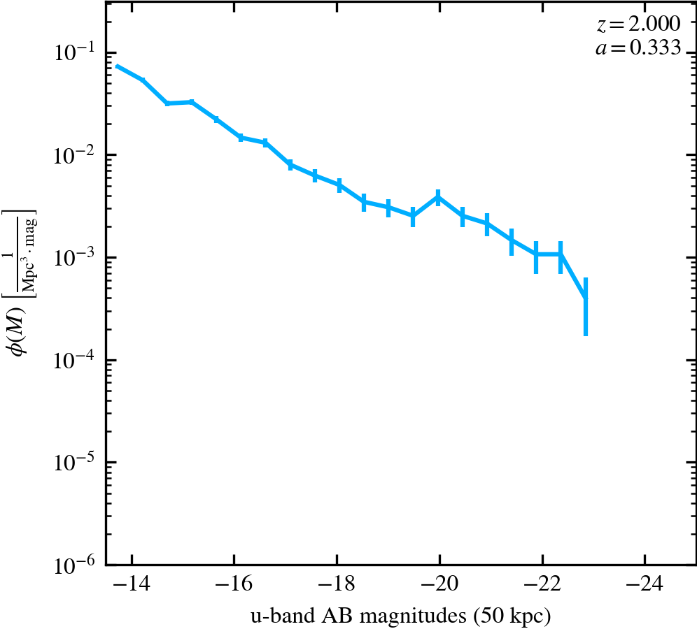
u-band Luminosity Function (50 kpc aperture)
50 kpc aperture dust-free rest-frame luminosity function in the GAMA u-band, constructed using the Trayford et al. (2015) model, showing all galaxies with a fixed bin-width of 0.2 dex.
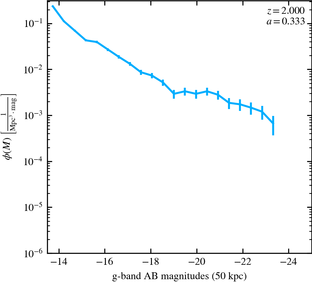
g-band Luminosity Function (50 kpc aperture)
50 kpc aperture dust-free rest-frame luminosity function in the GAMA g-band, constructed using the Trayford et al. (2015) model, showing all galaxies with a fixed bin-width of 0.2 dex.
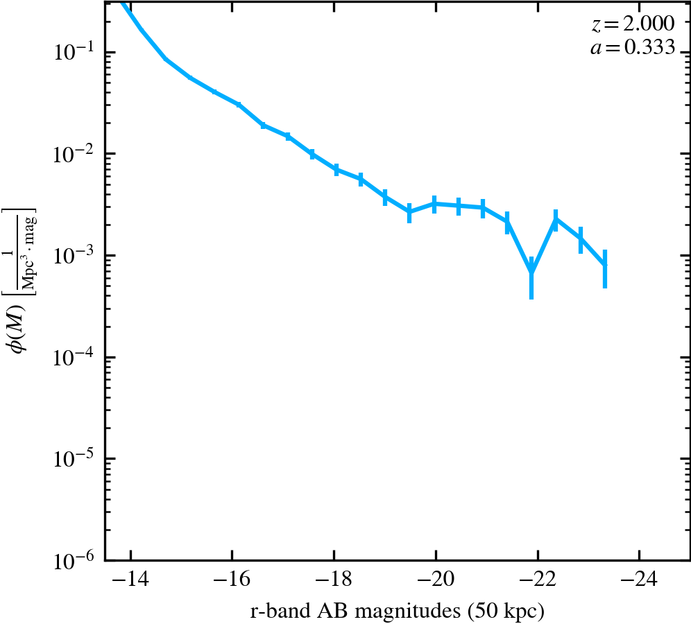
r-band Luminosity Function (50 kpc aperture)
50 kpc aperture dust-free rest-frame luminosity function in the GAMA r-band, constructed using the Trayford et al. (2015) model, showing all galaxies with a fixed bin-width of 0.2 dex.
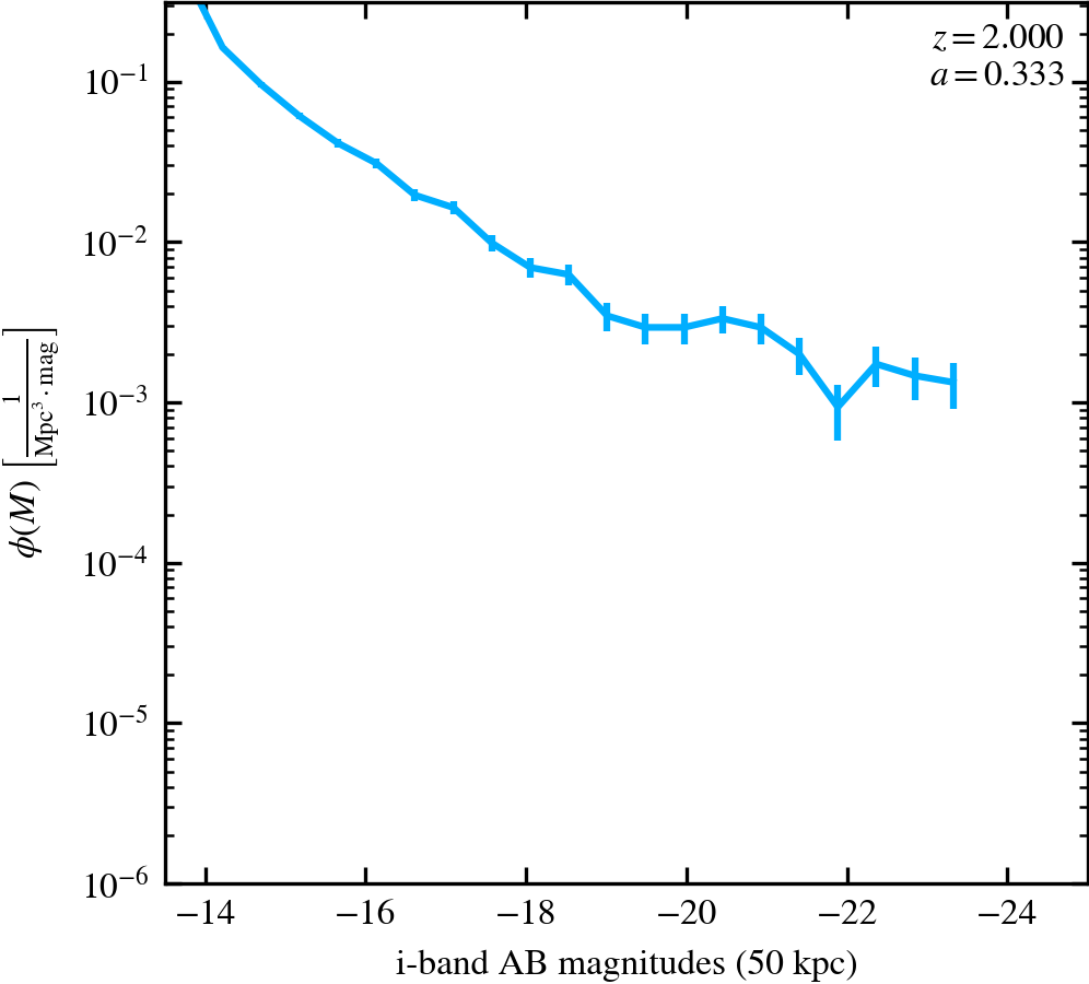
i-band Luminosity Function (50 kpc aperture)
50 kpc aperture dust-free rest-frame luminosity function in the GAMA i-band, constructed using the Trayford et al. (2015) model, showing all galaxies with a fixed bin-width of 0.2 dex.
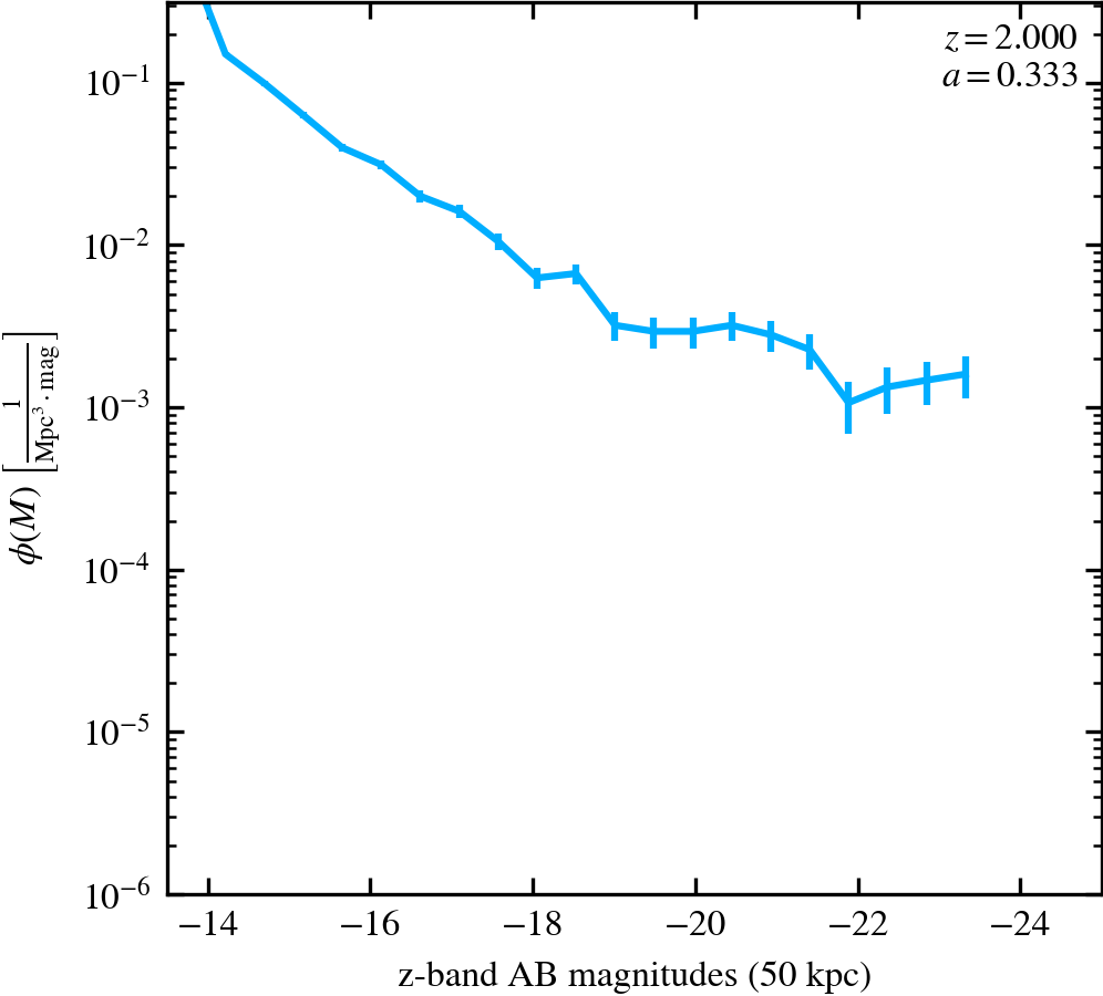
z-band Luminosity Function (50 kpc aperture)
50 kpc aperture dust-free rest-frame luminosity function in the GAMA z-band, constructed using the Trayford et al. (2015) model, showing all galaxies with a fixed bin-width of 0.2 dex.
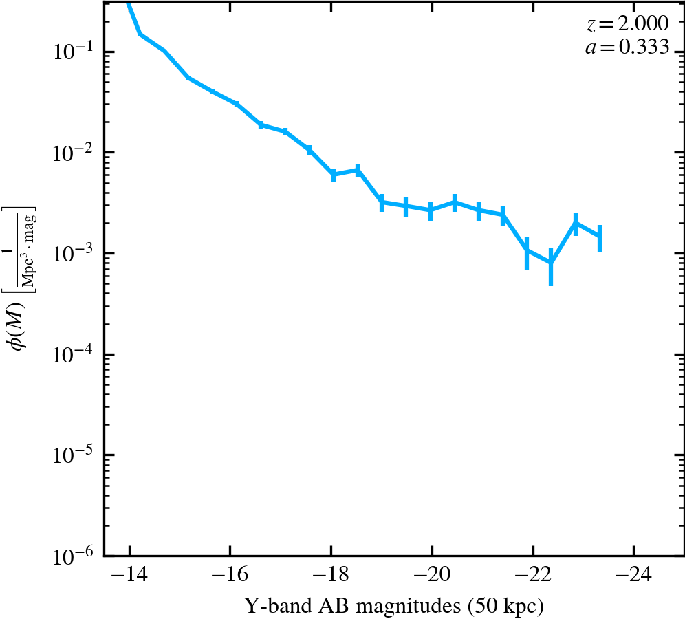
Y-band Luminosity Function (50 kpc aperture)
50 kpc aperture dust-free rest-frame luminosity function in the GAMA Y-band, constructed using the Trayford et al. (2015) model, showing all galaxies with a fixed bin-width of 0.2 dex.
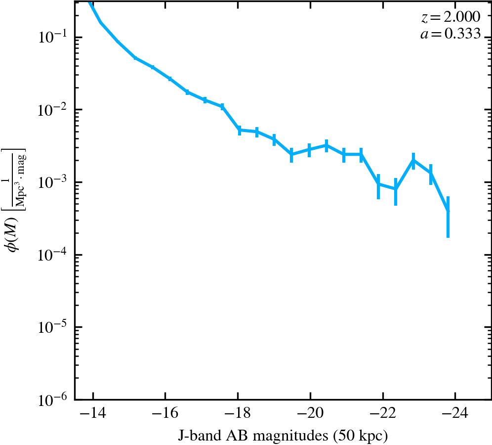
J-band Luminosity Function (50 kpc aperture)
50 kpc aperture dust-free rest-frame luminosity function in the GAMA J-band, constructed using the Trayford et al. (2015) model, showing all galaxies with a fixed bin-width of 0.2 dex.
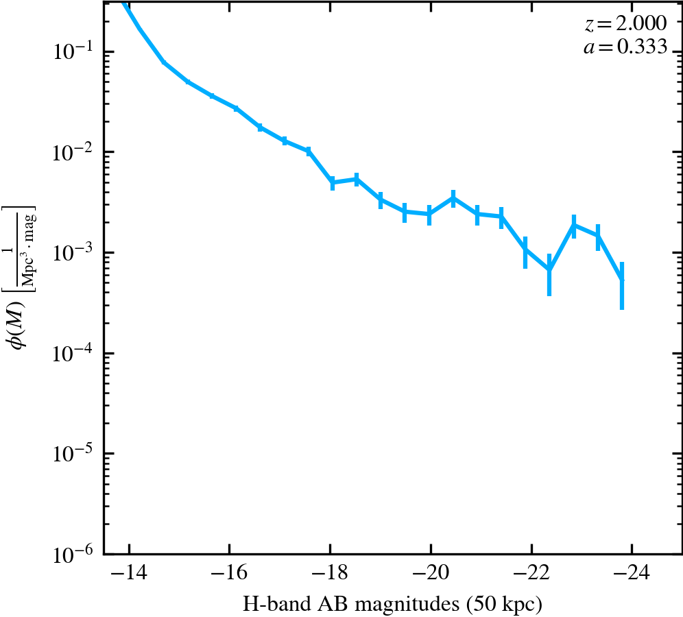
H-band Luminosity Function (50 kpc aperture)
50 kpc aperture dust-free rest-frame luminosity function in the GAMA H-band, constructed using the Trayford et al. (2015) model, showing all galaxies with a fixed bin-width of 0.2 dex.
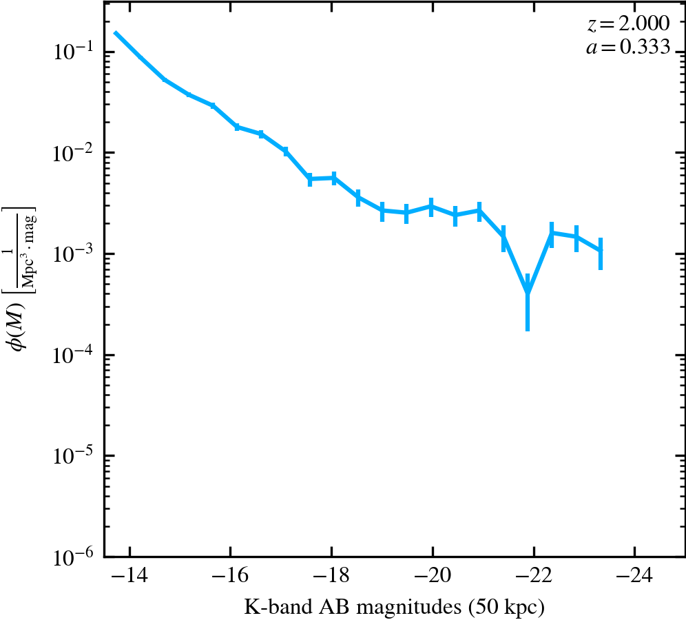
K-band Luminosity Function (50 kpc aperture)
50 kpc aperture dust-free rest-frame luminosity function in the GAMA K-band, constructed using the Trayford et al. (2015) model, showing all galaxies with a fixed bin-width of 0.2 dex.
Maximal Temperatures
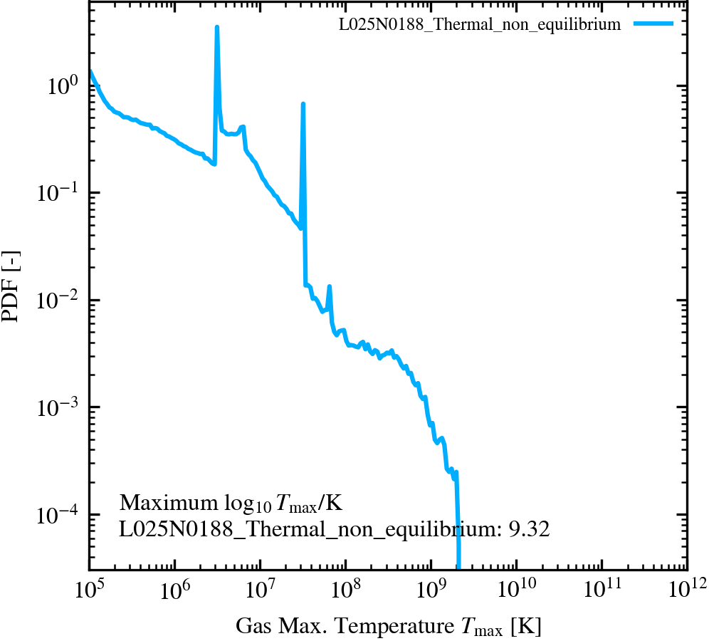
Maximal Temperature reached by gas particles
Maximal temperature recorded by gas particles throughout the entire simulation.
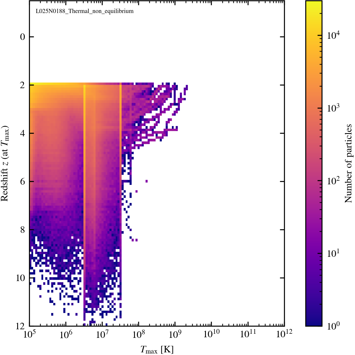
Maximal Temperature-Redshift
The maximal temperatures reached by all star and gas particles (density given by the colour map) against the redshift at which they were at that temperature.
Metal Evolution
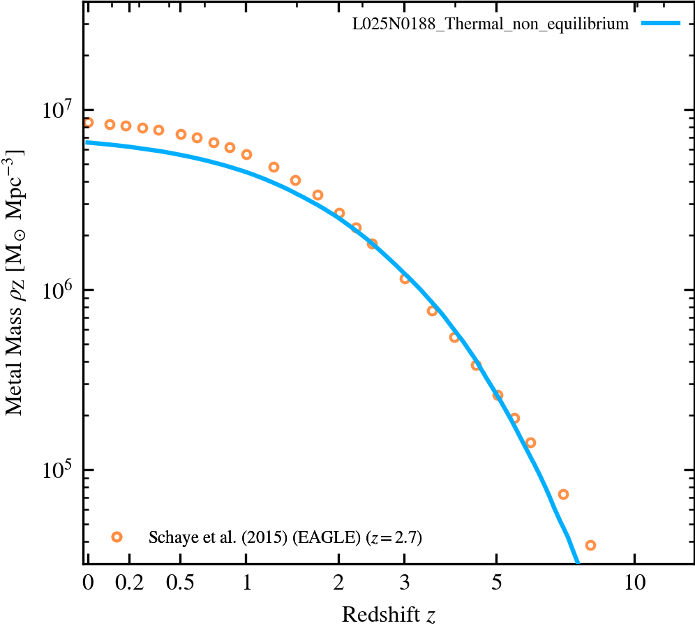
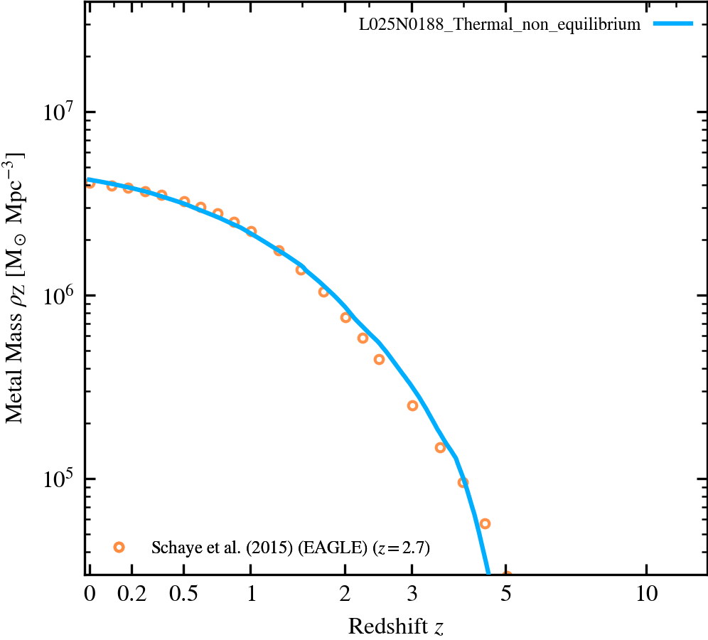
Gas Phase Metal Mass Density Evolution
Evolution of the metal mass in gas per unit co-moving volume.
Metal Mass Locked in Stars Density Evolution
Evolution of the metal mass locked in stars per unit co-moving volume.
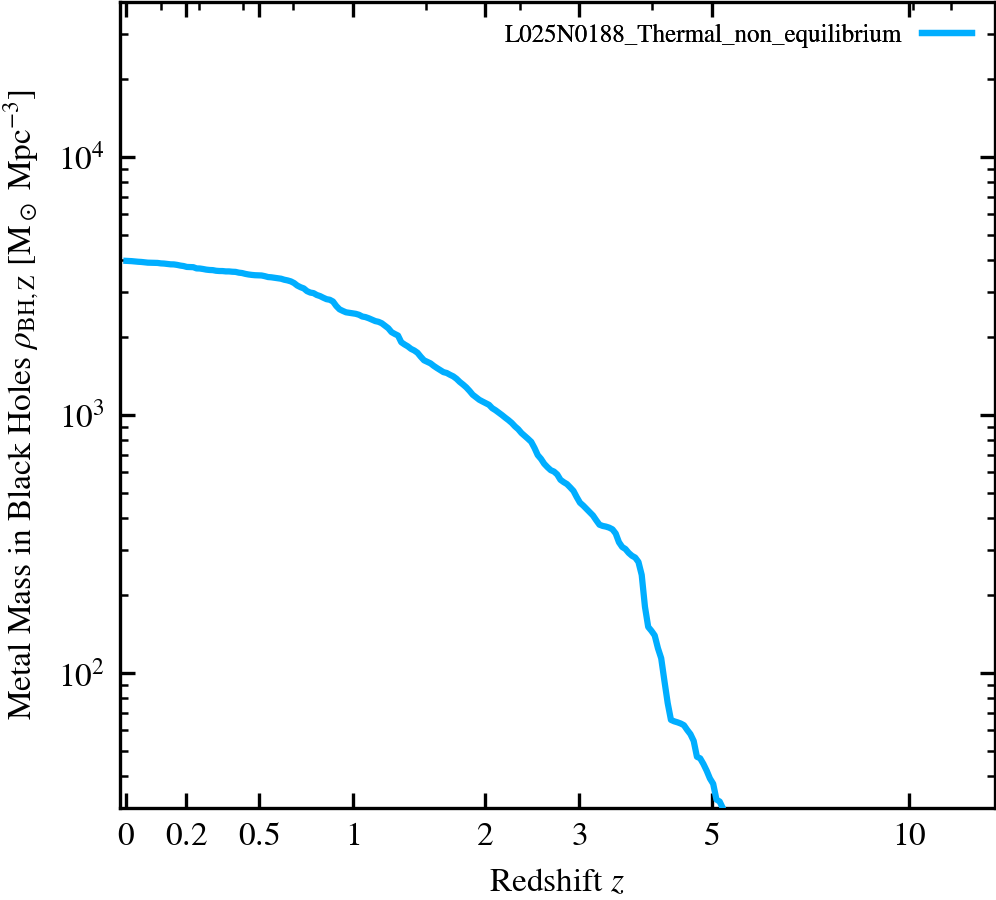
Metal Mass Locked in Black Holes Density Evolution
Evolution of the metal mass locked in black holes per unit co-moving volume.
Metal Mass Fractions
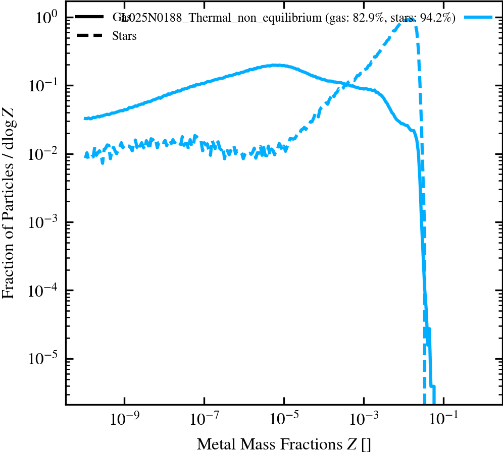
Metal Mass Fraction Distribution
Metal mass fraction distribution shown for each simulation; solid lines show gas metallicity and dashed lines show the same for the stars. If present, dashed line represents the entropy floor (equation of state). The percentages in between brackets indicate what fraction of the particles is above the lower limit and hence included in the distribution.
Run Performance
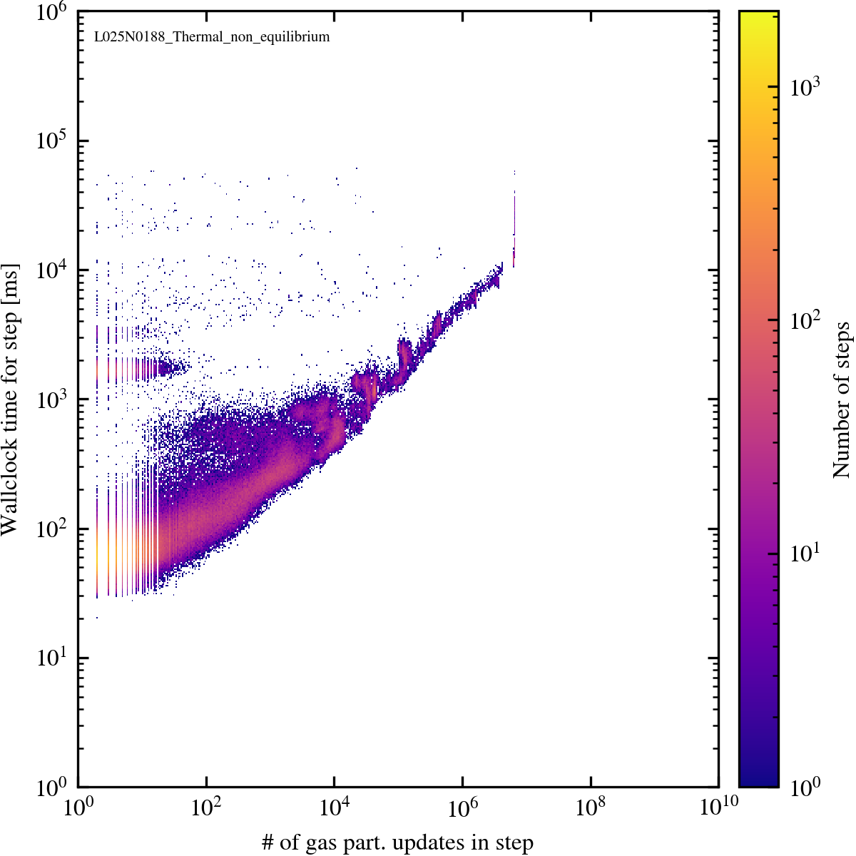
Wall-clock time per gas particle updates.
Wall-clock time to run a time-step as a function of the number of gas particles updated. The tracks at the top correspond to steps where the tree is rebuilt, i/o is performed, FoF is run or other non-regular operations are done.
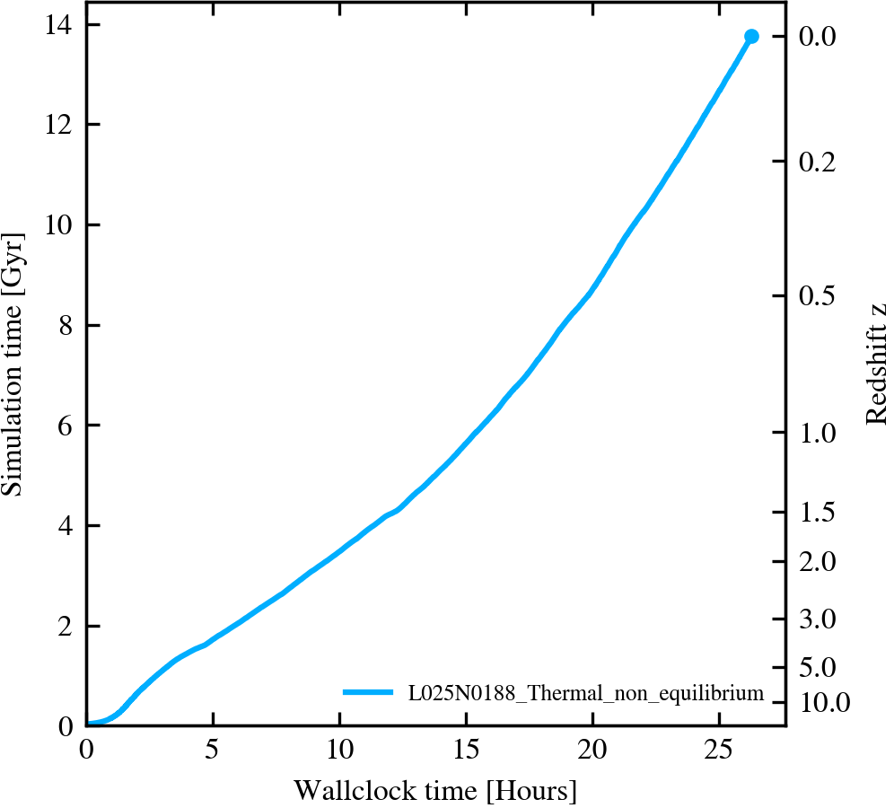
Cosmic time vs. wall-clock time
The cosmic time as a function of the wall-clock time.
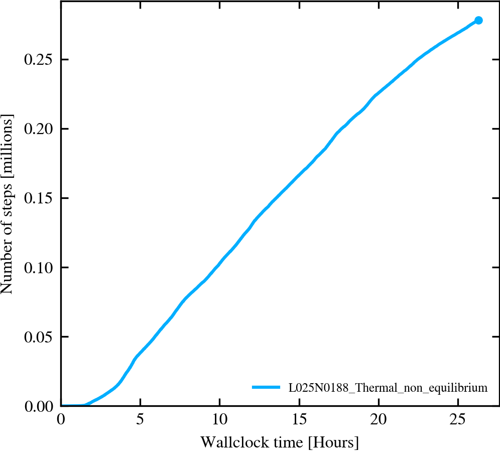
The number of steps vs. wall-clock time
The cumulative number of the simulation time-steps as a function of the wall-clock time.
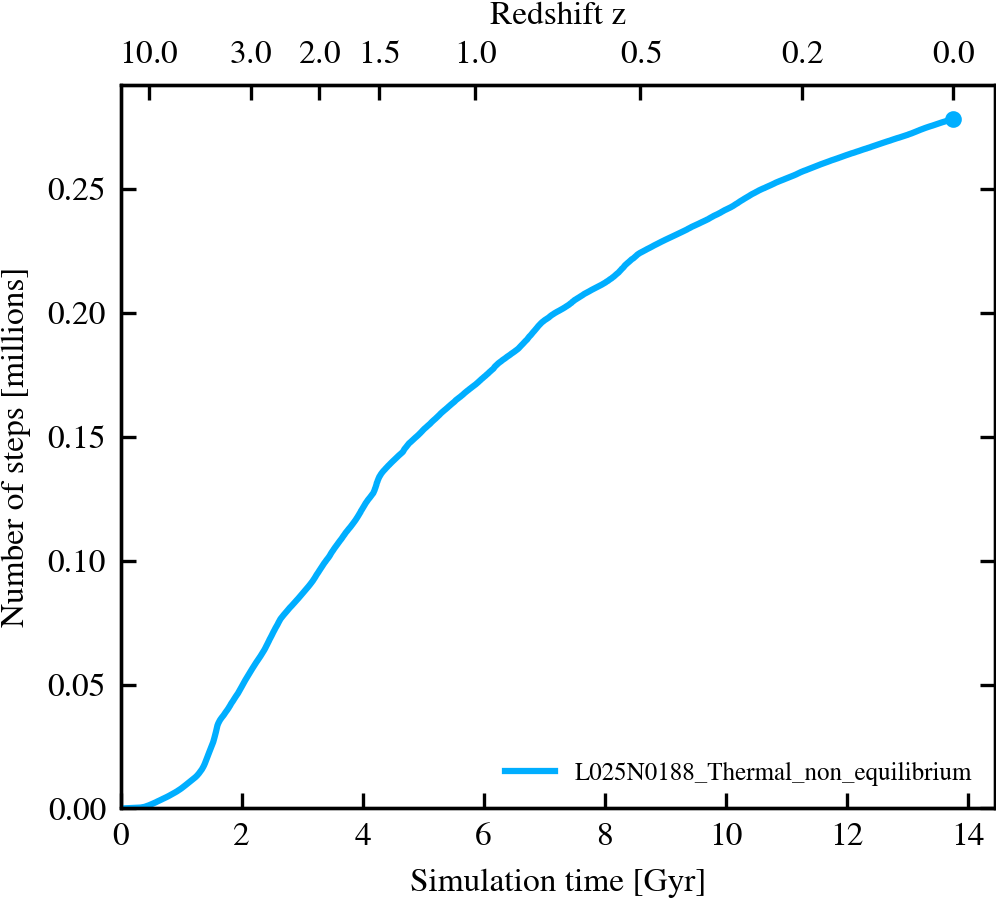
Number of steps vs. cosmic time
The cumulative number of the simulation time-steps as a function of the cosmic time.
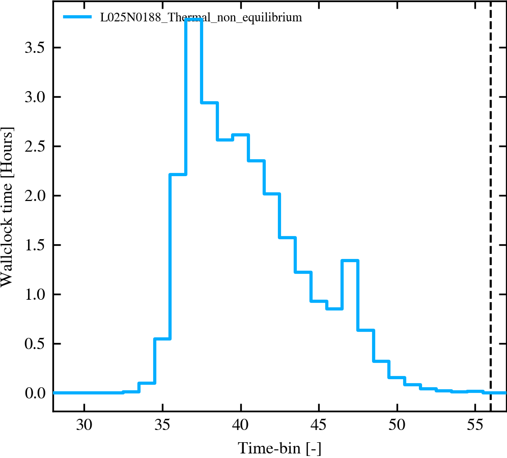
Wall-clock time per time-bin
Total wall-clock time spent in each of the different simulation time-bins.
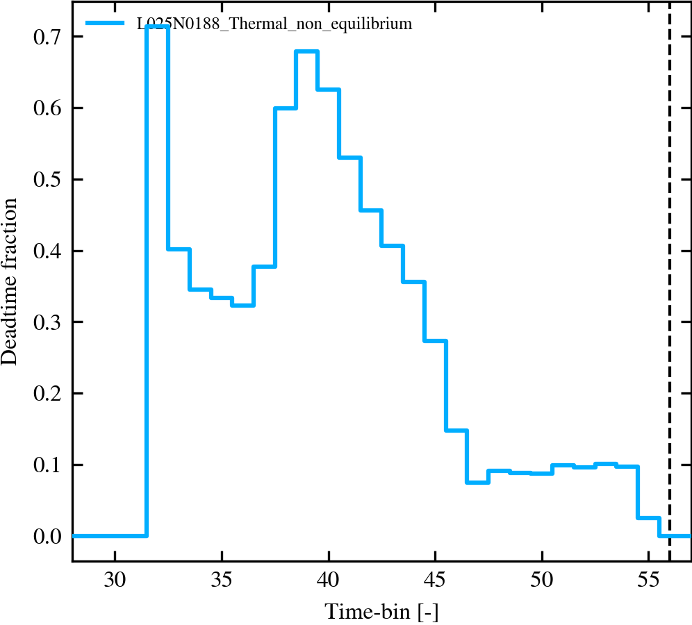
Deadtime fraction per time-bin
Dead time fraction in each simulation time-bin.
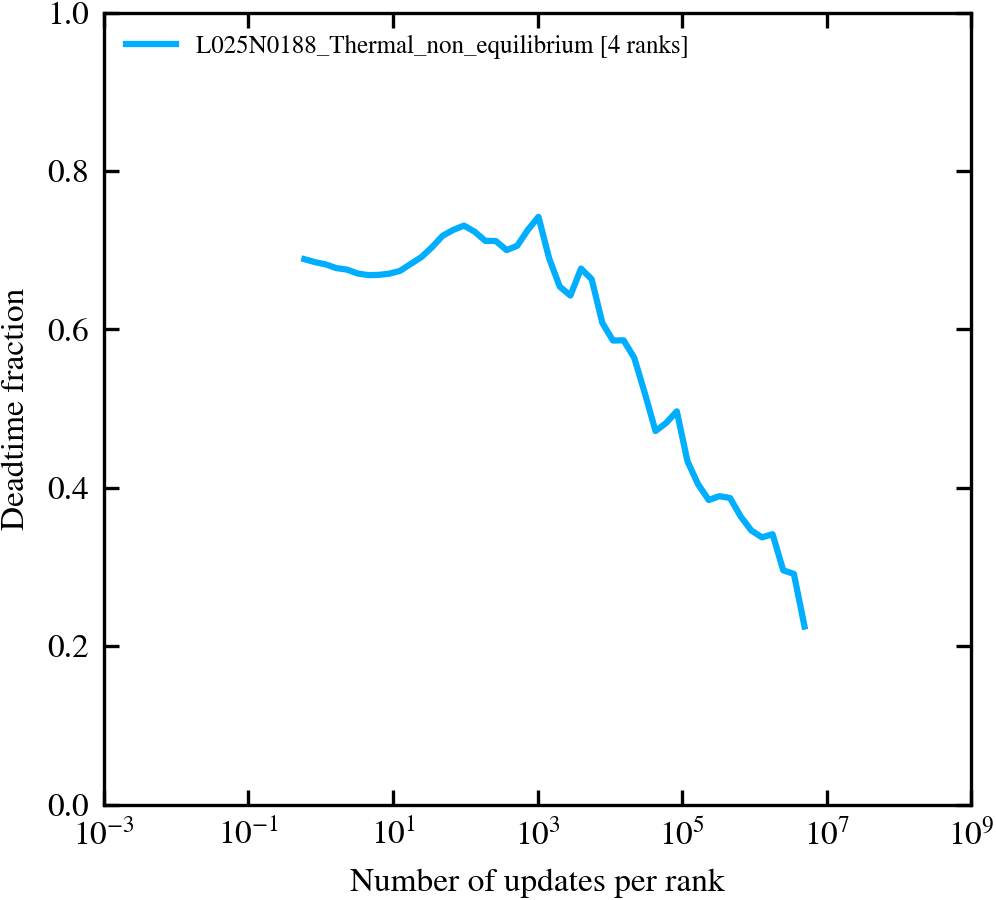
Step size vs deadtime fraction
Dead time fraction as a function of number of updates per rank.
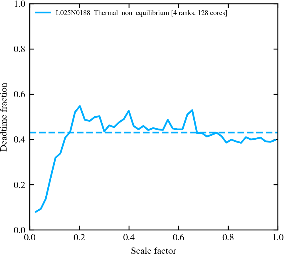
Dead time fraction vs scale factor
Evolution of the dead time fraction as a function of scale factor. The dashed line represents the average dead time over the entire run.
Satellite Fraction
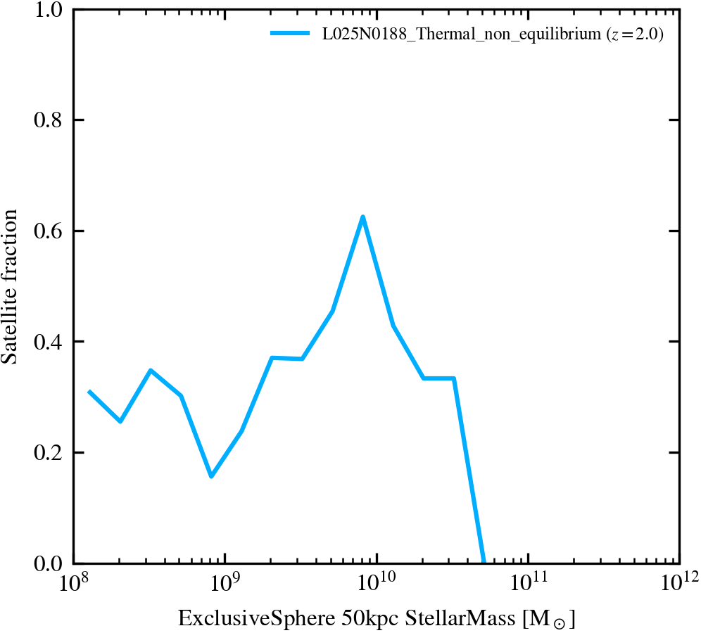
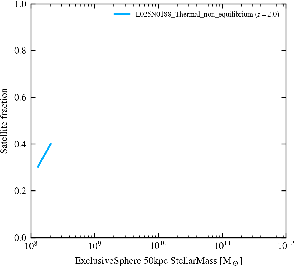
Satellite Fraction
The fraction of galaxies which are satellites as a function of their stellar mass
Satellite Fraction (Passive galaxies)
The fraction of passive galaxies which are satellites as a function of their stellar mass
Sizes
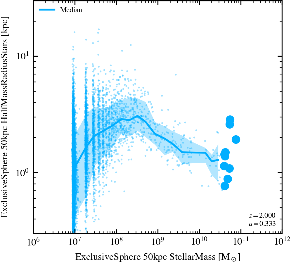
Stellar Mass-Galaxy Size relation (50 kpc aperture)
Uses a 50 kpc 3D aperture.
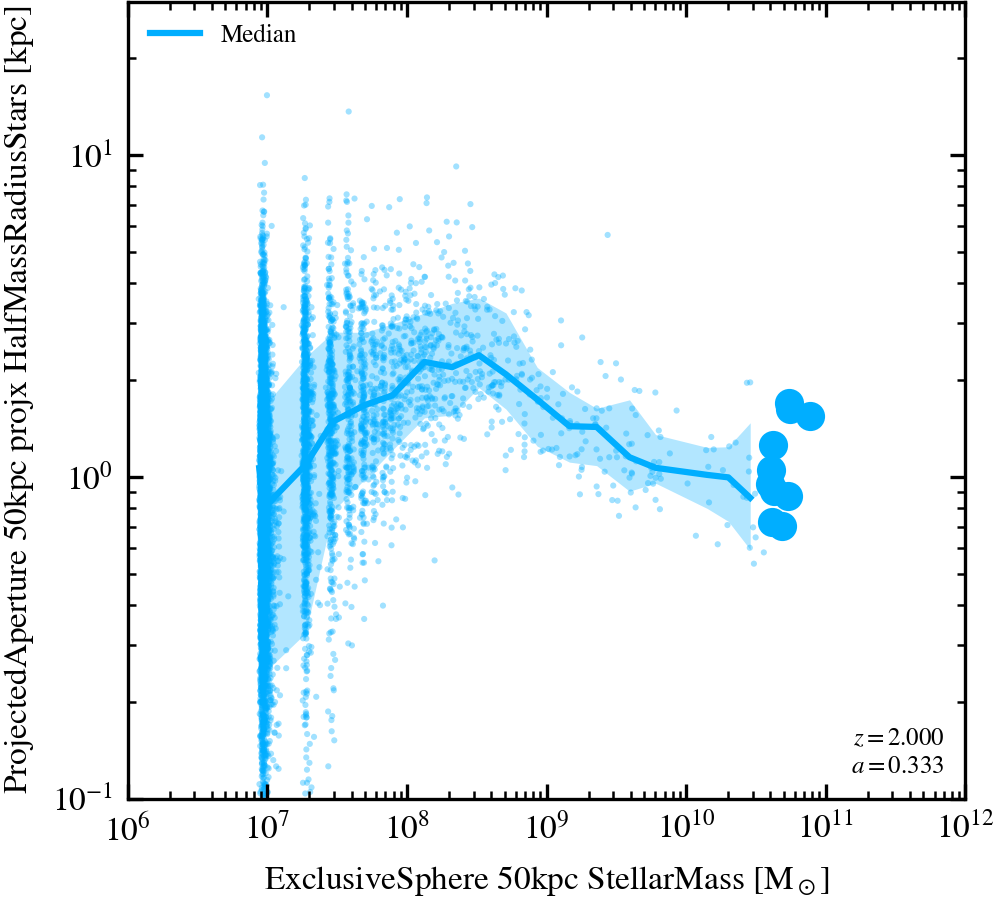
Stellar Mass-(Projected) Galaxy Size relation (50 kpc aperture)
Uses stellar sizes calculated from a projected distribution within a 50 kpc aperture.
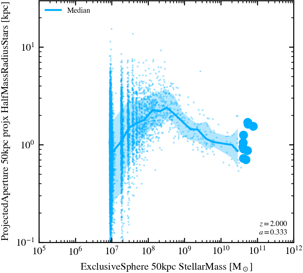
Stellar Mass-(Projected) Galaxy Size relation (50 kpc aperture, calibration)
Uses stellar sizes calculated from a projected distribution within a 50 kpc aperture. The comparison data is used for calibration.
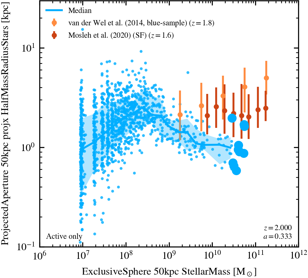
Stellar Mass-(Projected) Galaxy Size relation (50 kpc aperture)
Only shows active galaxies defined based on their sSFRs. Both Lange et al. (2015) and van der Wel et al. (2014) use the semi-major half-light radius of the best-fitting Sérsic model as the definition of galaxy size, while Mosleh et al. (2020) use the circularized half-light radius.
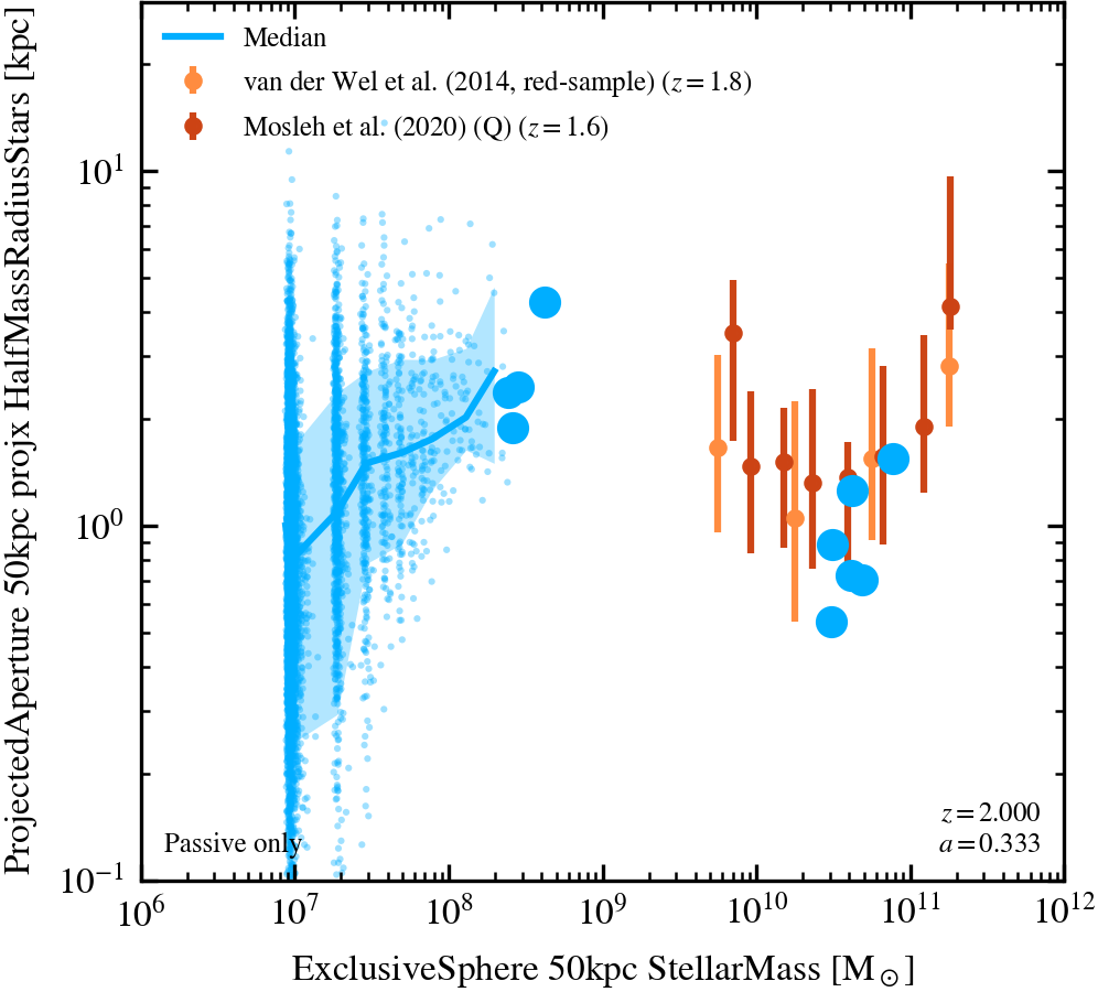
Stellar Mass-(Projected) Galaxy Size relation (50 kpc aperture)
Only shows passive galaxies defined based on their sSFRs. Both Lange et al. (2015) and van der Wel et al. (2014) use the semi-major half-light radius of the best-fitting Sérsic model as the definition of galaxy size, while Mosleh et al. (2020) use the circularized half-light radius.
SN Feedback Energy Fractions
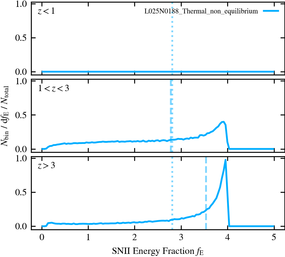
SNII Energy Fraction Distribution
Distribution of SNII energy fractions, split by redshift. The y-axis shows the number of stars per bin divided by the bin width and by the total number of stars. The dashed vertical lines show the median SNII energy fraction in three different redshift intervals. The dotted vertical line shows the average SNII energy fraction computed over all star particles in the simulation.
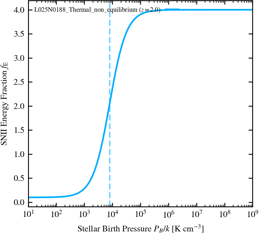
SNII Energy Fraction vs. Stellar Birth Pressure
The relation between the SNII energy fraction and stellar birth pressure. The dashed vertical lines indicate the pivot birth pressure used in the simulation.
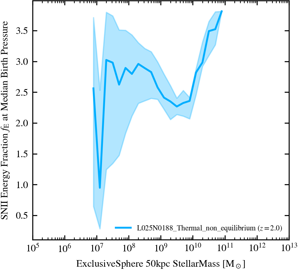
SNII Energy Fraction vs. Galaxy Stellar Mass
The SNII energy fraction evaluated at the galaxy median stellar birth pressure vs. galaxy stellar mass. The solid lines indicate the median values in stellar mass bins, while the shaded regions indicate the 16-84 percentile scatter.
SNIa Rate
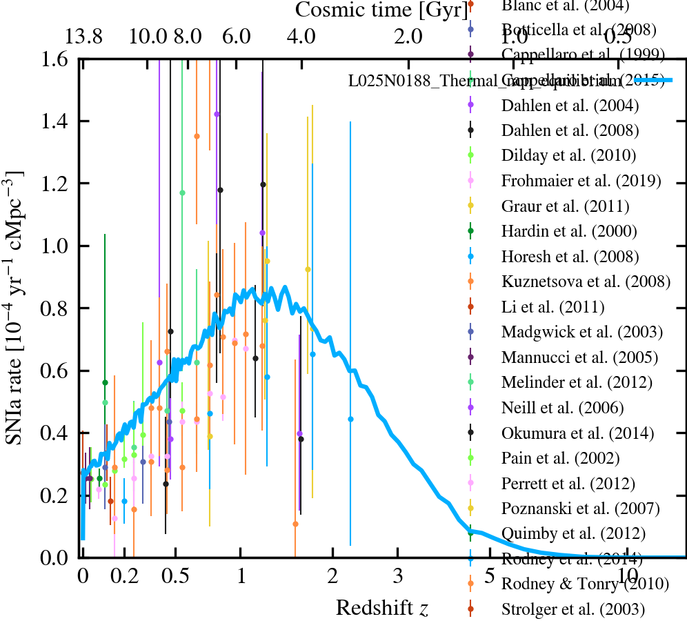
Cosmic SNIa rate
SNIa rate history plotted directly from the SNIa.txt file produced by SWIFT.
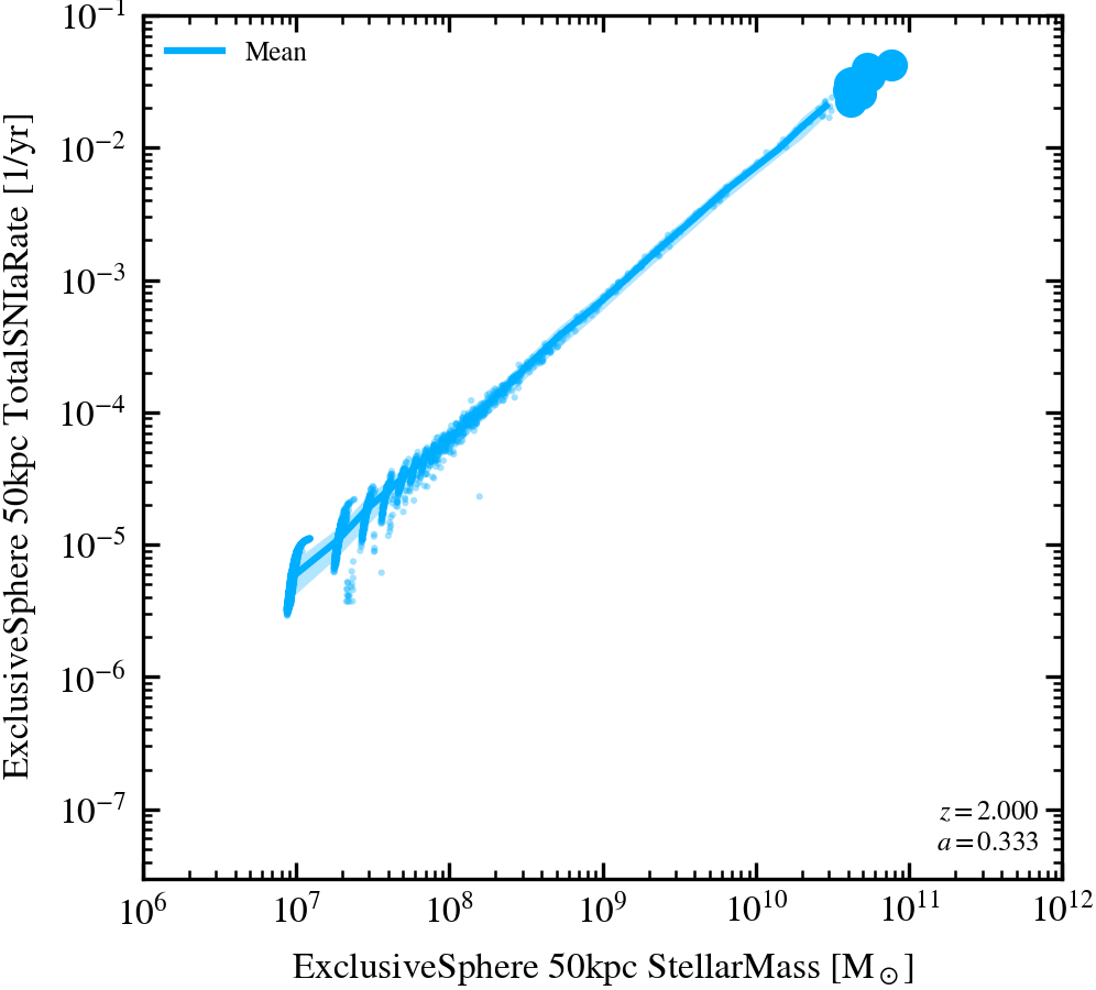
Stellar Mass-SNIa rate relation (50 kpc aperture)
Uses a 50 kpc 3D aperture.
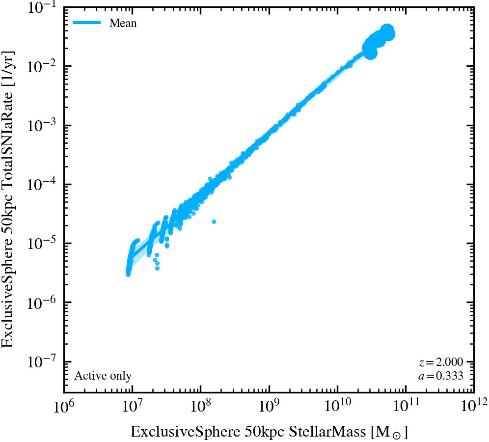
Stellar Mass-SNIa rate relation (active only, 50 kpc aperture)
Uses a 50 kpc 3D aperture and only active galaxies.
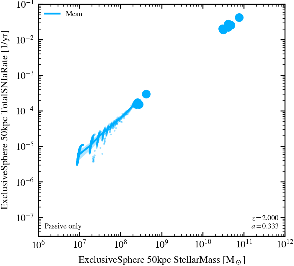
Stellar Mass-SNIa rate relation (passive only, 50 kpc aperture)
Uses a 50 kpc 3D aperture and only passive galaxies.
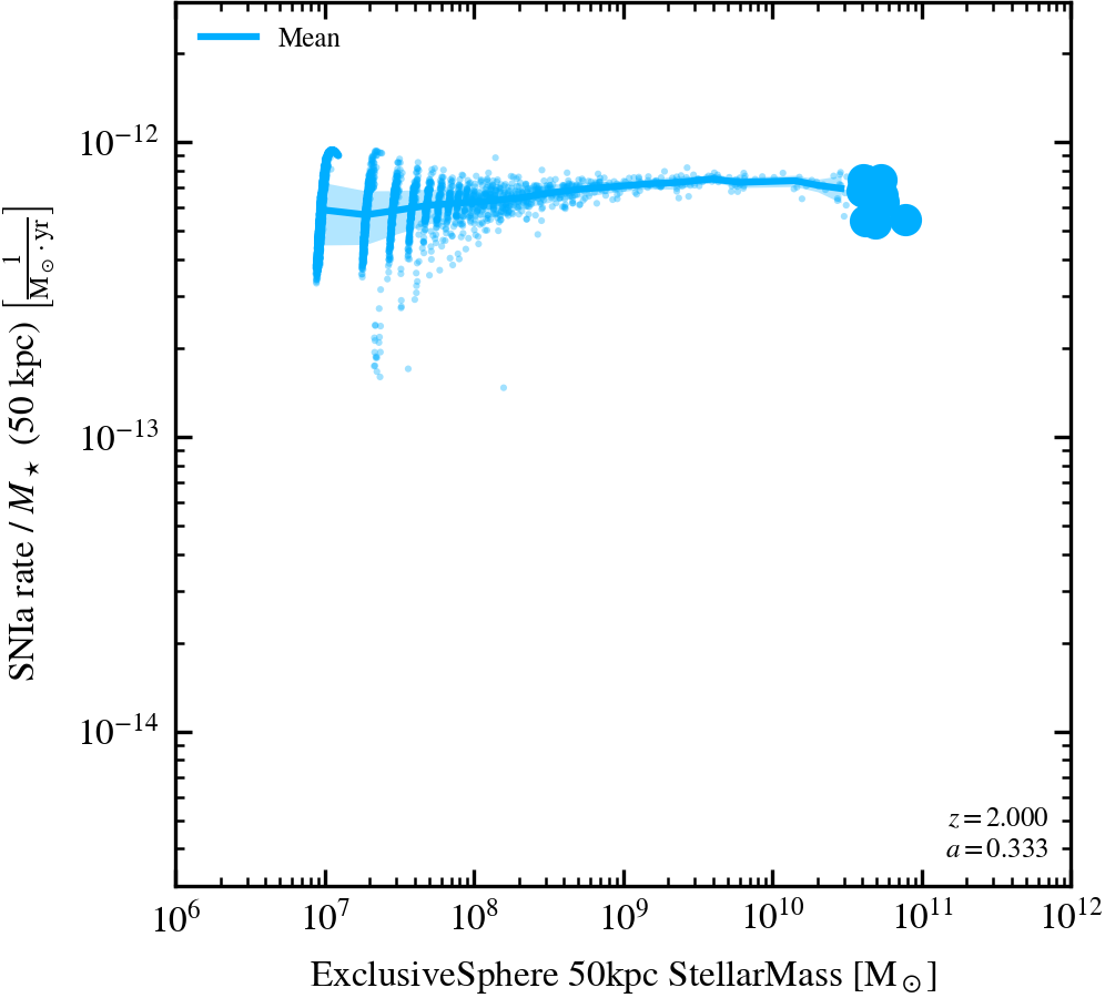
Stellar Mass-SNIa rate per stellar mass relation (50 kpc aperture)
Uses a 50 kpc 3D aperture.
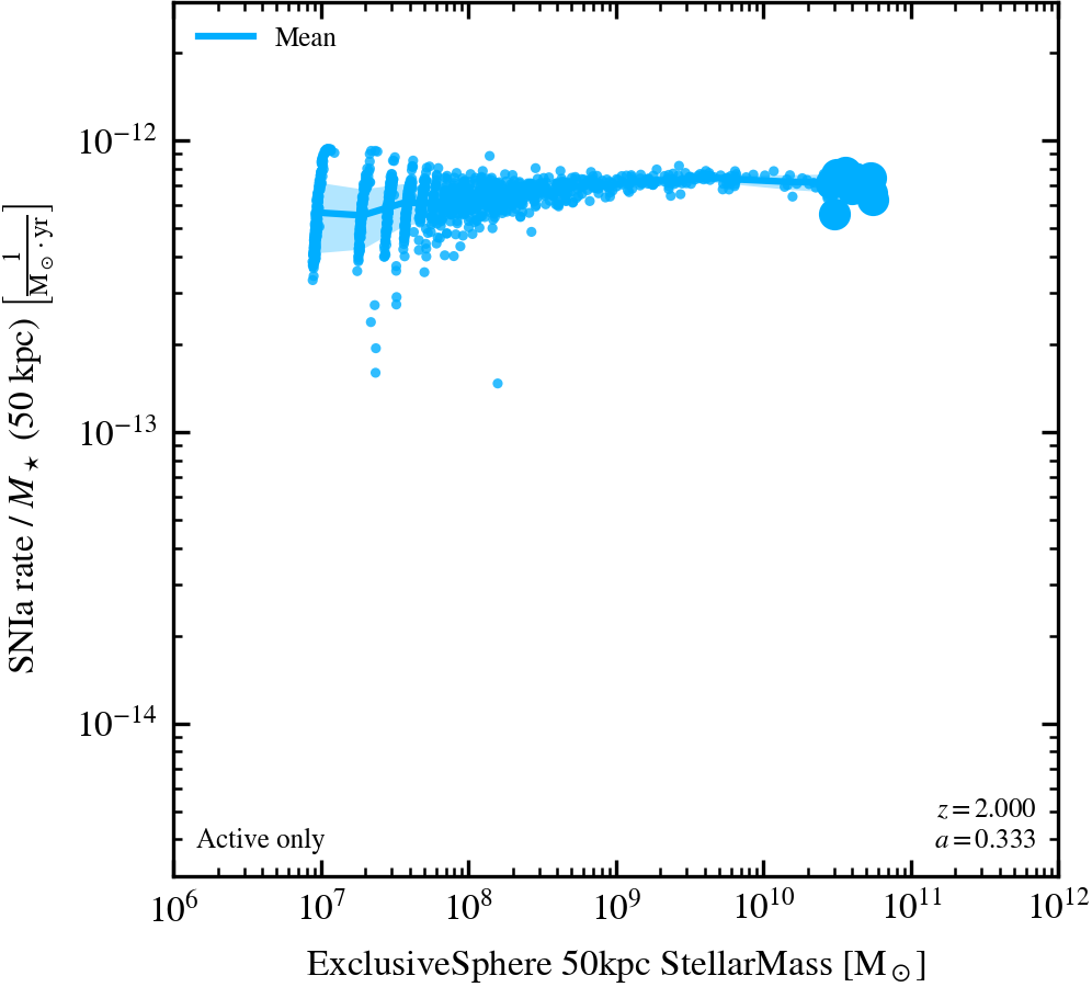
Stellar Mass-SNIa rate per stellar mass relation (active only, 50 kpc aperture)
Uses a 50 kpc 3D aperture.
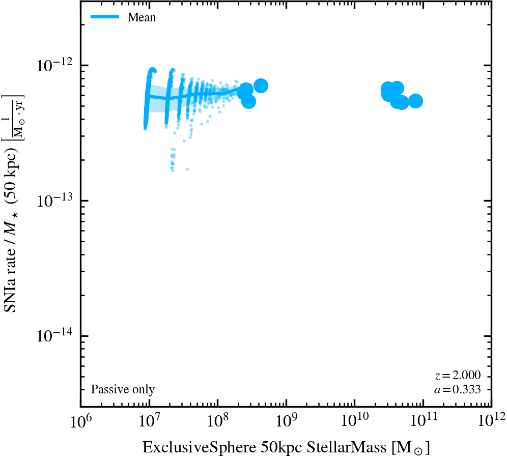
Stellar Mass-SNIa rate per stellar mass relation (passive only, 50 kpc aperture)
Uses a 50 kpc 3D aperture.
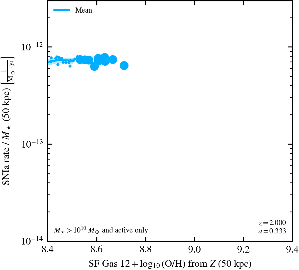
Gas metallicity-SNIa rate per stellar mass relation (active only, 50 kpc aperture)
Uses a 50 kpc 3D aperture, active galaxies only with a stellar mass above 1e10 Msun.
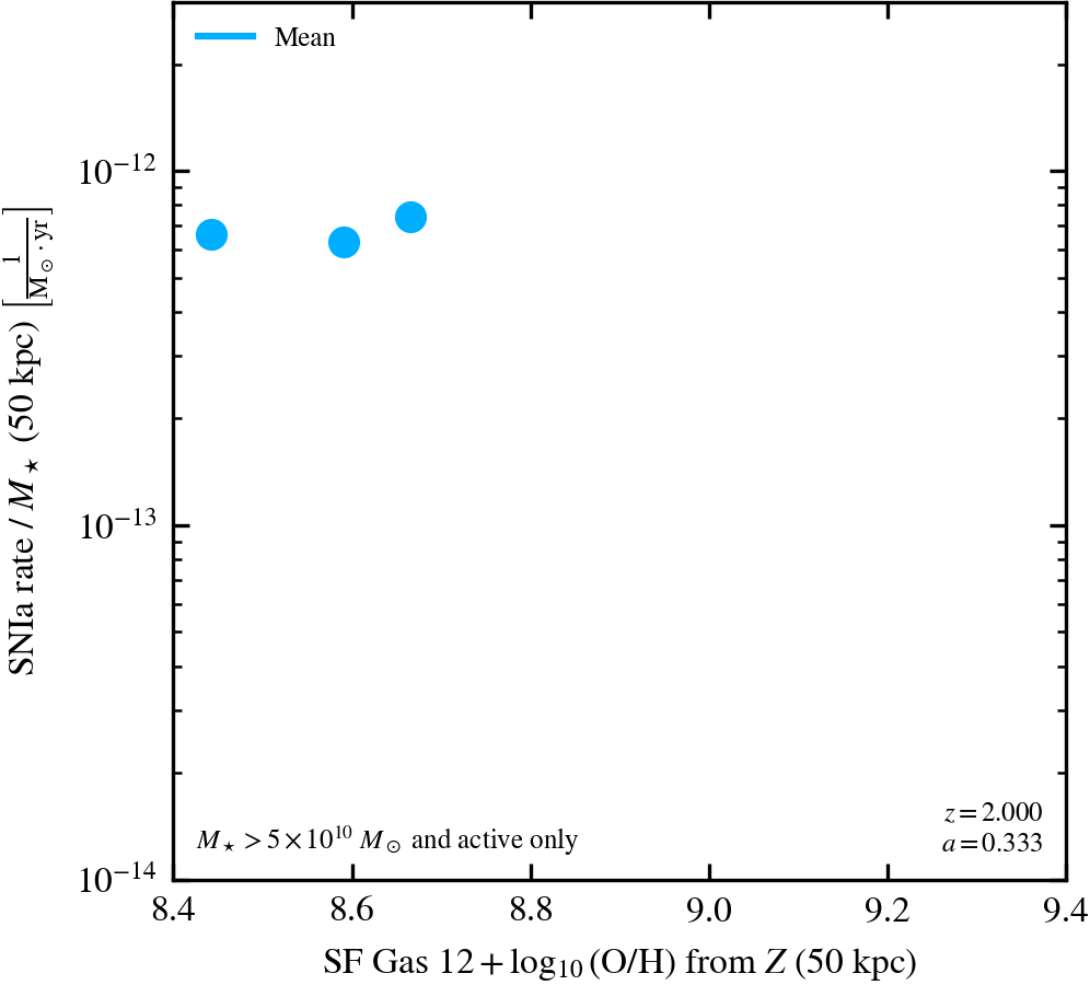
Gas metallicity-SNIa rate per stellar mass relation (active only, 50 kpc aperture)
Uses a 50 kpc 3D aperture, active galaxies only with a stellar mass above 5e10 Msun.
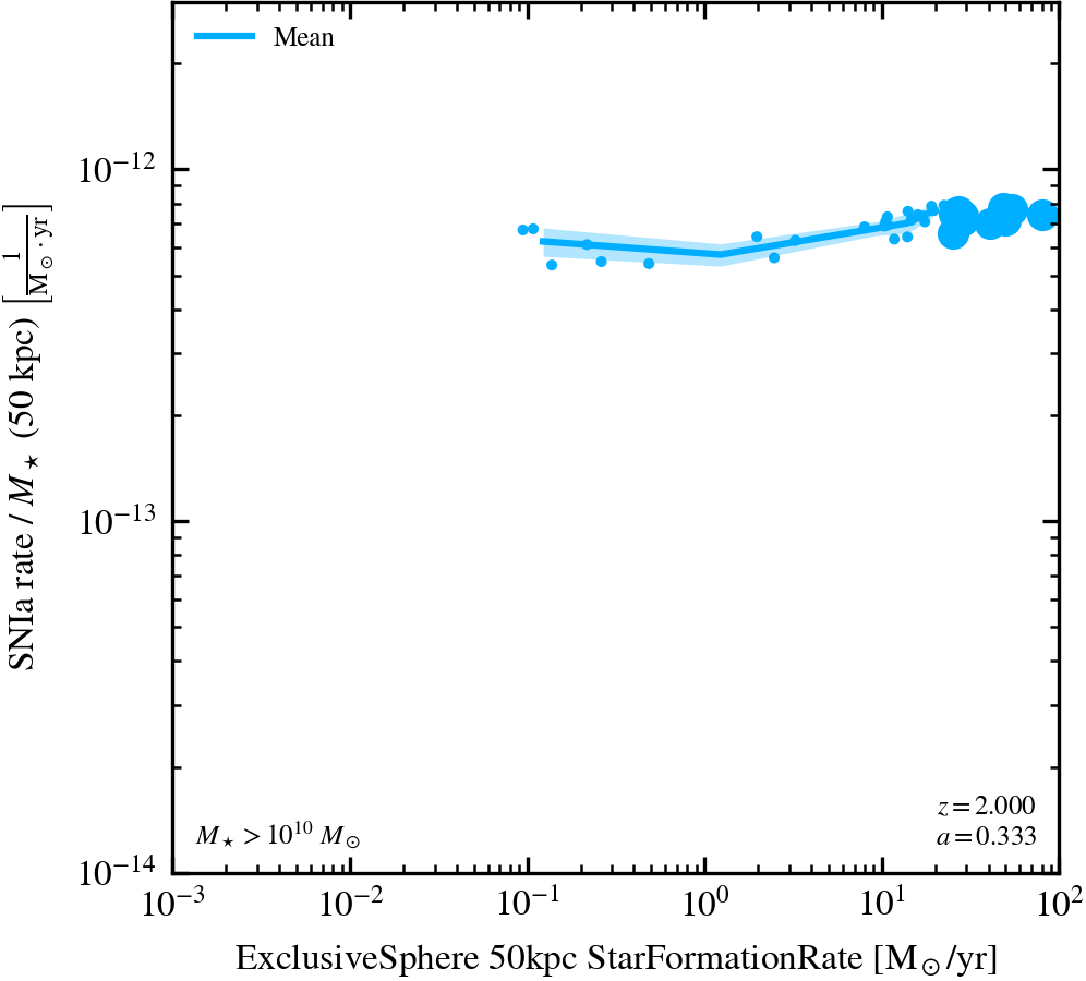
SFR-SNIa rate per stellar mass relation (50 kpc aperture)
Uses a 50 kpc 3D aperture, only select galaxies with a stellar mass above 1e10 Msun.
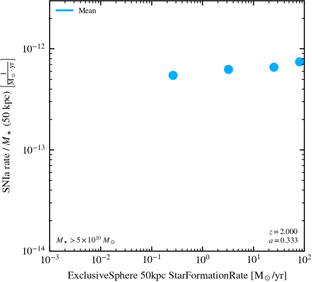
SFR-SNIa rate per stellar mass relation (50 kpc aperture)
Uses a 50 kpc 3D aperture, only select galaxies with a stellar mass above 5e10 Msun.
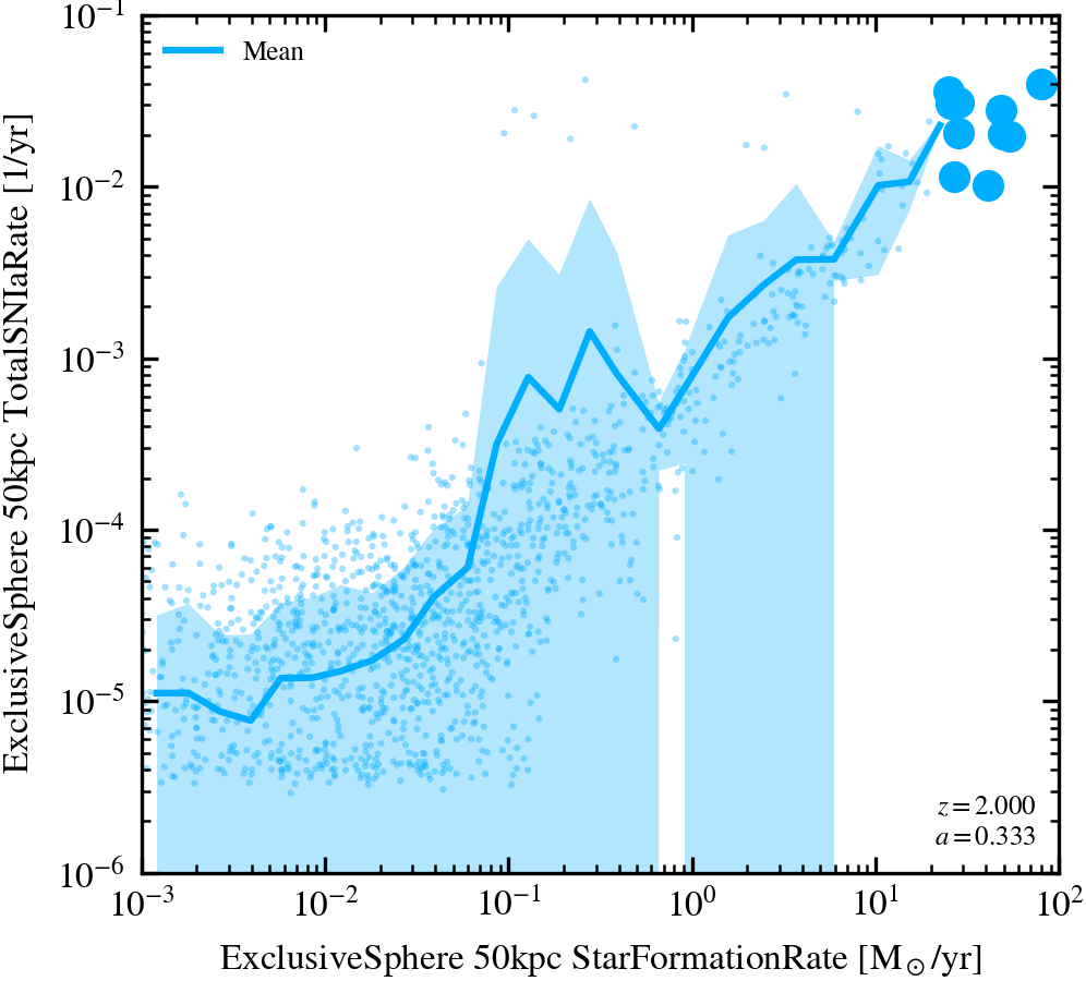
SFR-SNIa rate relation (50 kpc aperture)
Uses a 50 kpc 3D aperture.
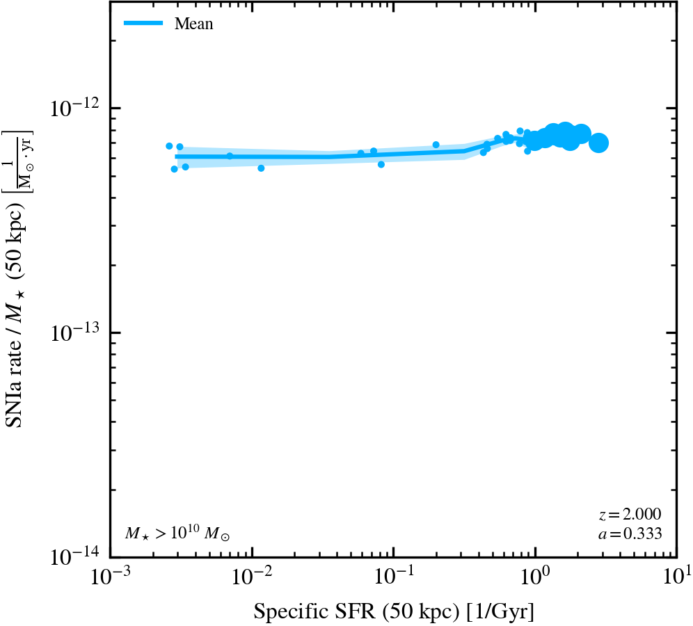
sSFR-SNIa rate per stellar mass relation (50 kpc aperture)
Uses a 50 kpc 3D aperture, only select galaxies with a stellar mass above 1e10 Msun.
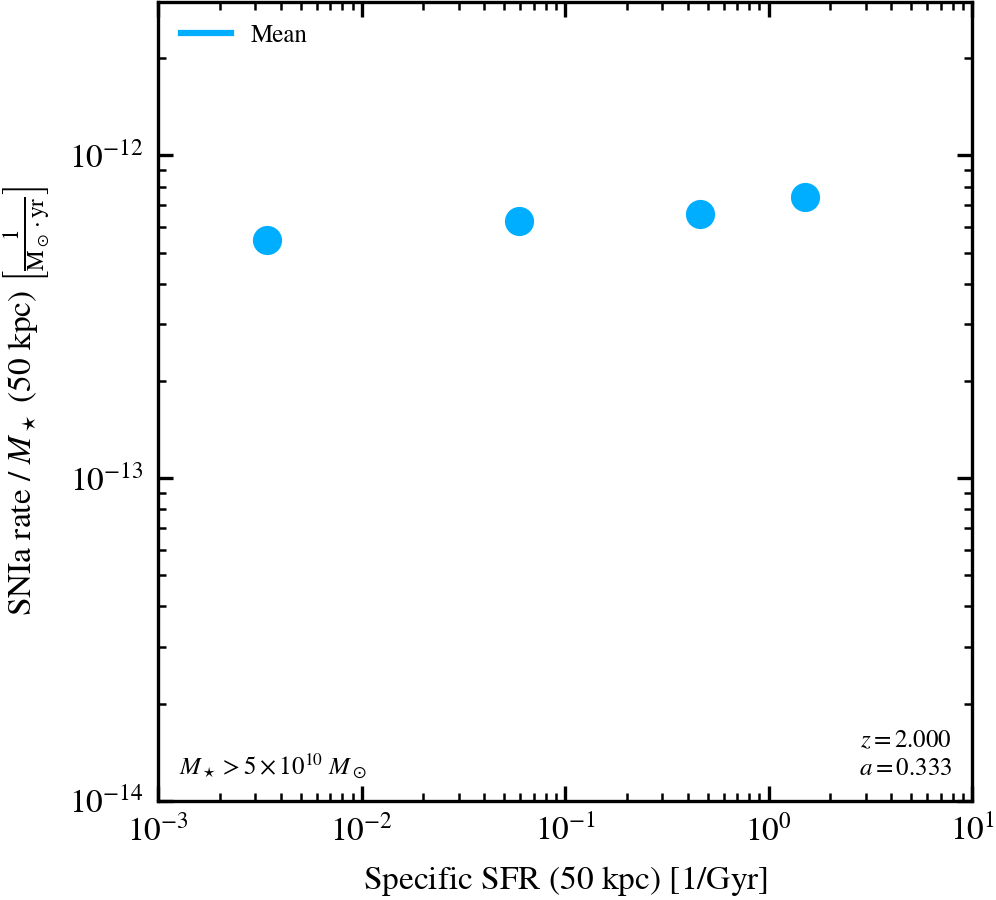
sSFR-SNIa rate per stellar mass relation (50 kpc aperture)
Uses a 50 kpc 3D aperture, only select galaxies with a stellar mass above 5e10 Msun.
Star Formation Density History
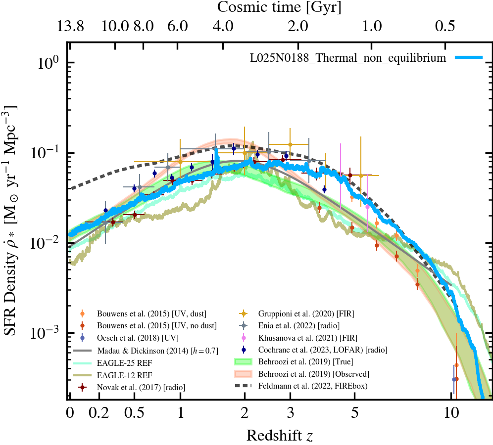
Star Formation History
Star formation density history plotted directly from the SFR.txt file produced by SWIFT.
Star Formation History
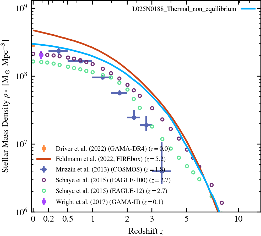
Stellar Mass Density Evolution
Evolution of the stellar mass density plotted directly from the statistics.txt file produced by SWIFT.
Star Formation Rates
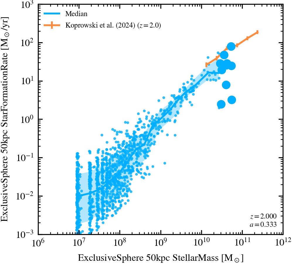
Stellar Mass-Star Formation Rate (50 kpc aperture) for active galaxies.
Only active galaxies are included. SFRs from Koprowski+ are based on UV+IV; active galaxies in Koprowski+ were identified based on UVJ colour selection.
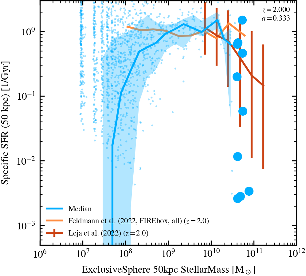
Specific Star Formation Rate - Stellar Mass (50 kpc aperture)
All galaxies, including those deemed to be passive (z=0 sSFR threshold is 0.01 / Gyr, z>0 is 0.2/t_H(z)), are included in the median line.
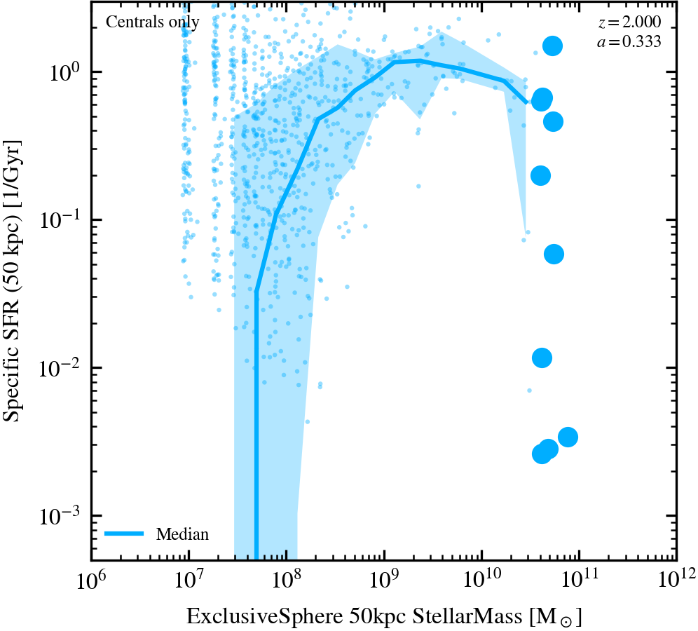
Specific Star Formation Rate - Stellar Mass (50 kpc aperture, centrals only)
Only central galaxies are included in the median line.
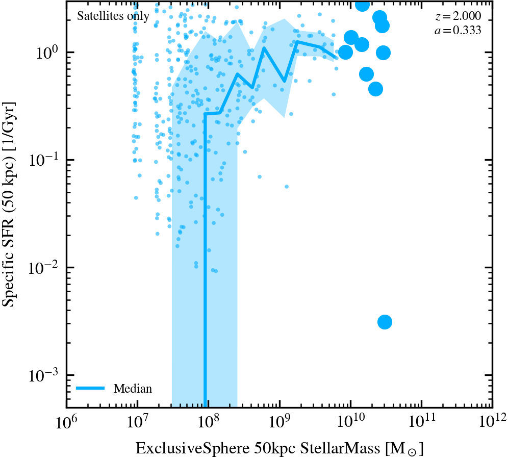
Specific Star Formation Rate - Stellar Mass (50 kpc aperture, satellites only)
Only satellite galaxies are included in the median line.
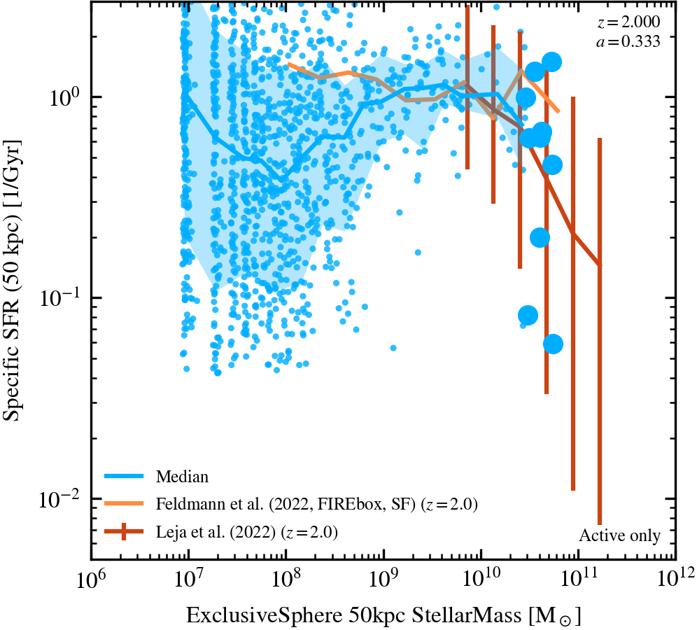
Specific Star Formation Rate - Stellar Mass (50 kpc aperture, active only)
Only active galaxies (z=0 sSFR threshold is 0.01 / Gyr, z>0 is 0.2/t_H(z)) are included in the median line.
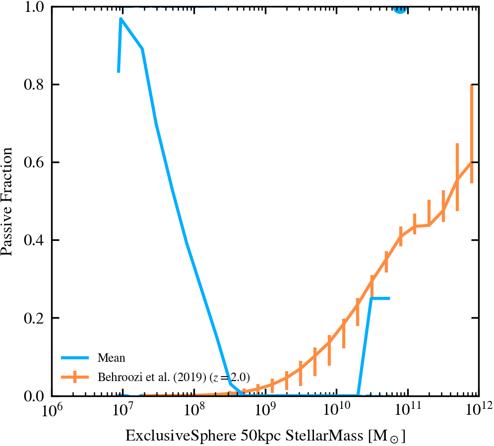
Passive Fraction - Stellar Mass (50 kpc aperture)
The sSFR threshold to determine if a galaxy is passsive is 0.01 / Gyr for z=0, 0.2/t_H(z) for z>0.
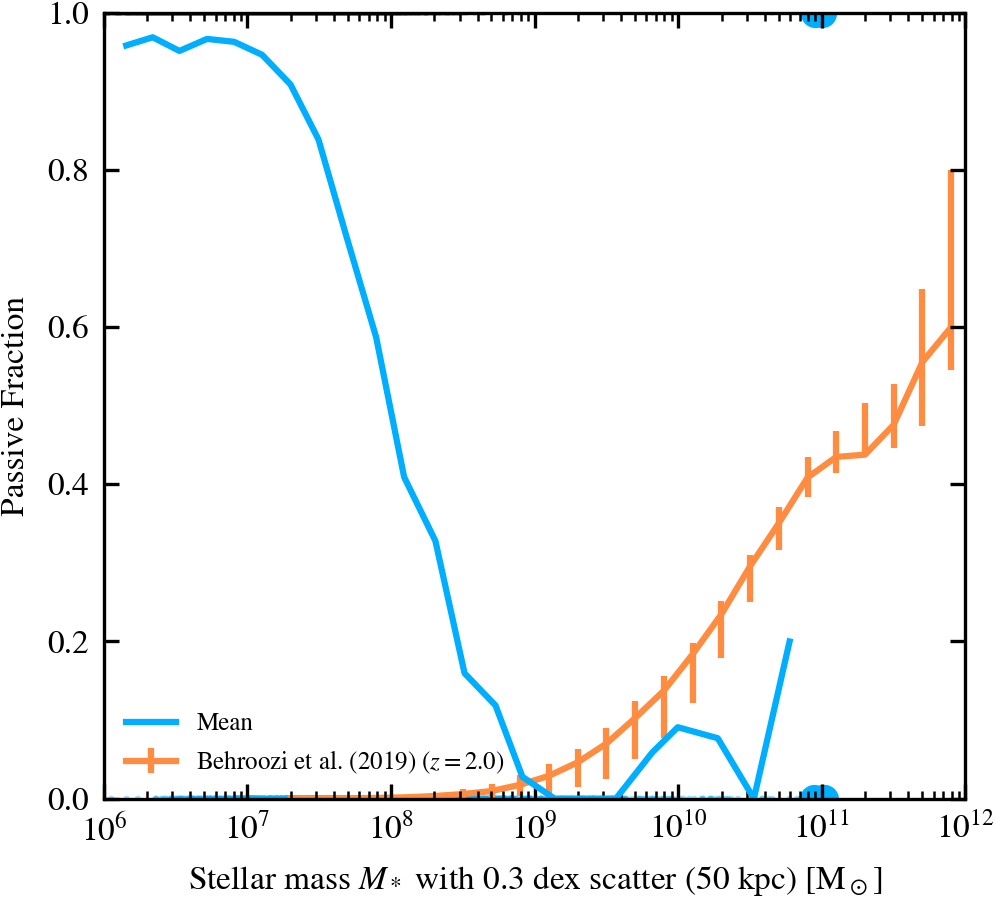
Passive Fraction - Stellar Mass (50 kpc aperture, with scatter)
The sSFR threshold to determine if a galaxy is passsive is 0.01 / Gyr for z=0, 0.2/t_H(z) for z>0. All stellar masses contain an additional 0.3 dex log-normal scatter.
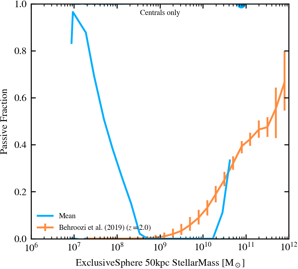
Passive Fraction - Stellar Mass (50 kpc aperture, centrals)
The sSFR threshold to determine if a galaxy is passsive is 0.01 / Gyr for z=0, 0.2/t_H(z) for z>0. This figure shows only central galaxies
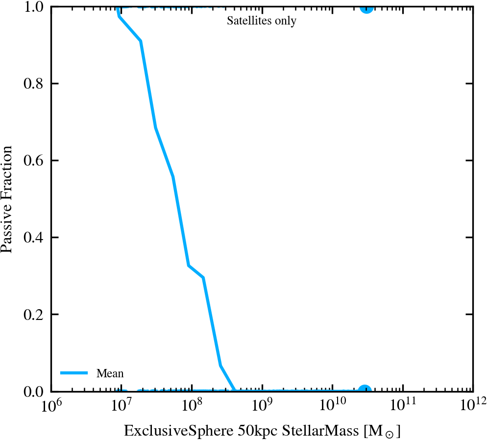
Passive Fraction - Stellar Mass (50 kpc aperture, satellites)
The sSFR threshold to determine if a galaxy is passsive is 0.01 / Gyr for z=0, 0.2/t_H(z) for z>0. This figure shows only satellite galaxies
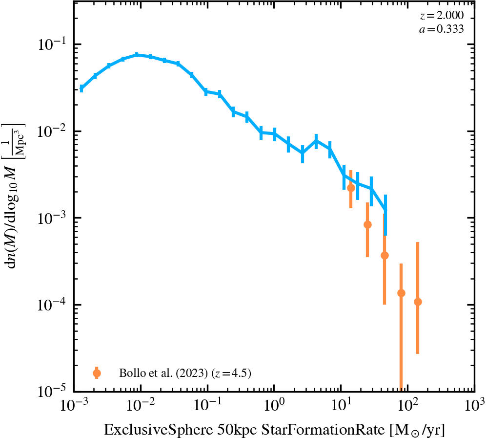
Star Formation Rate Function (50 kpc aperture)
50 kpc aperture galaxy star formation rate function, showing all galaxies with a fixed bin-width of 0.2 dex.
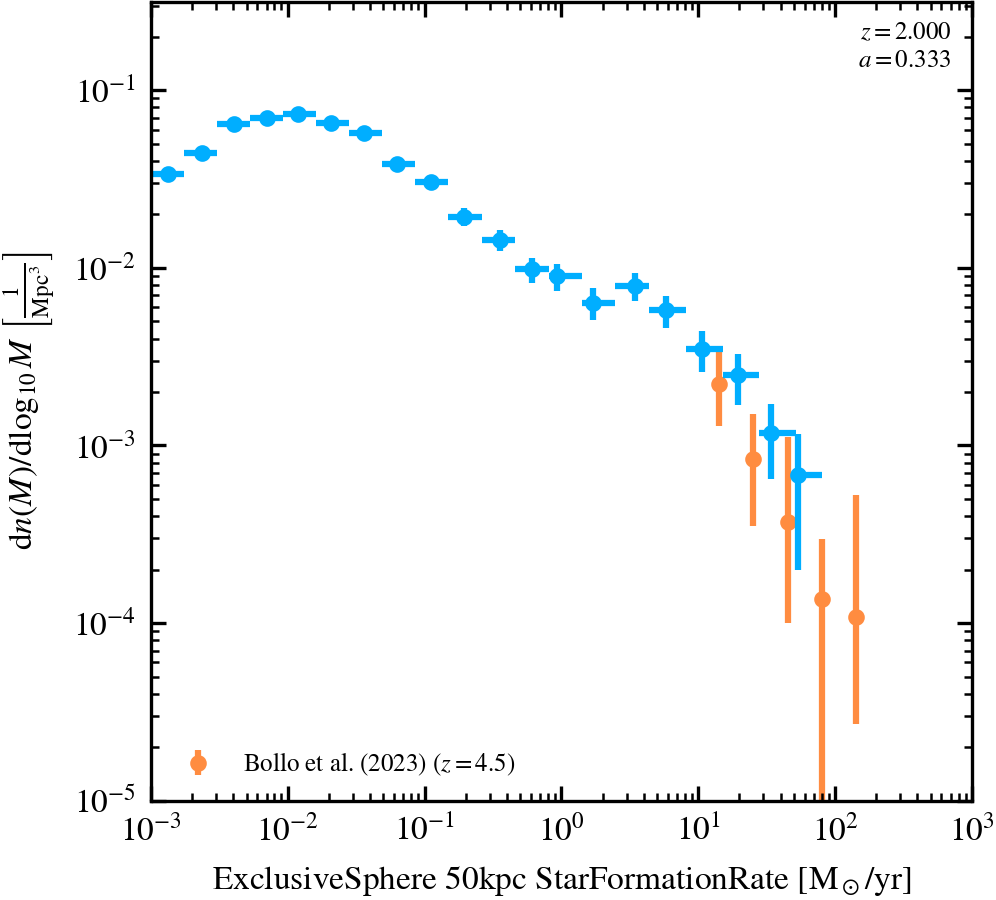
Star Formation Rate Function (50 kpc aperture)
50 kpc aperture galaxy star formation rate function, showing all galaxies with an adaptive bin-width.
Stellar Birth Properties
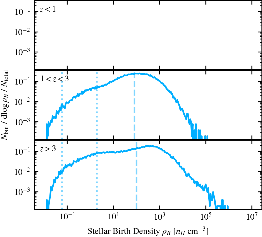
Stellar Birth Densities
Distributions of stellar birth densities, split by redshift. The y axis shows the number of stars per bin divided by the bin width and by the total number of stars. The dashed vertical lines show the median stellar birth-densities, while the dotted lines indicade the critical density from C. Dalla Vecchia & J. Schaye (2012) for SN min and max heating temperatures with $f_t=10$.
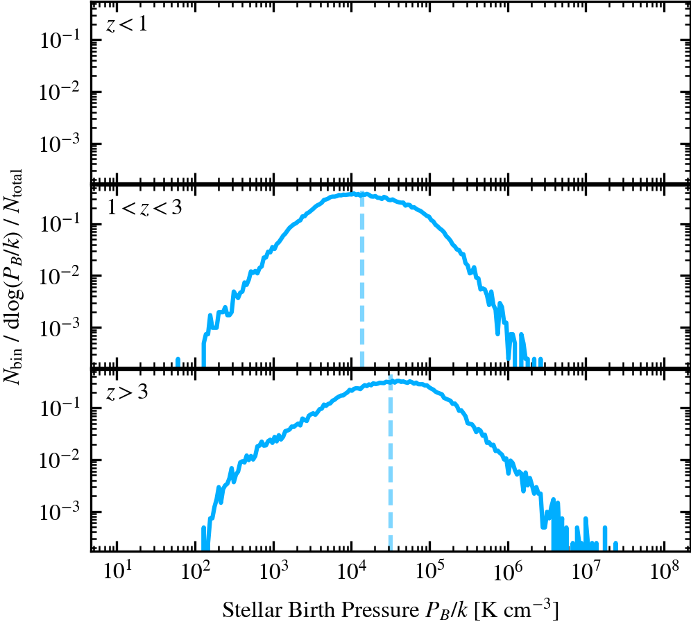
Stellar Birth Pressures
Distributions of stellar birth pressures, split by redshift. The y axis shows the number of stars per bin divided by the bin width and by the total number of stars. The dashed vertical lines show the median stellar birth-pressures.
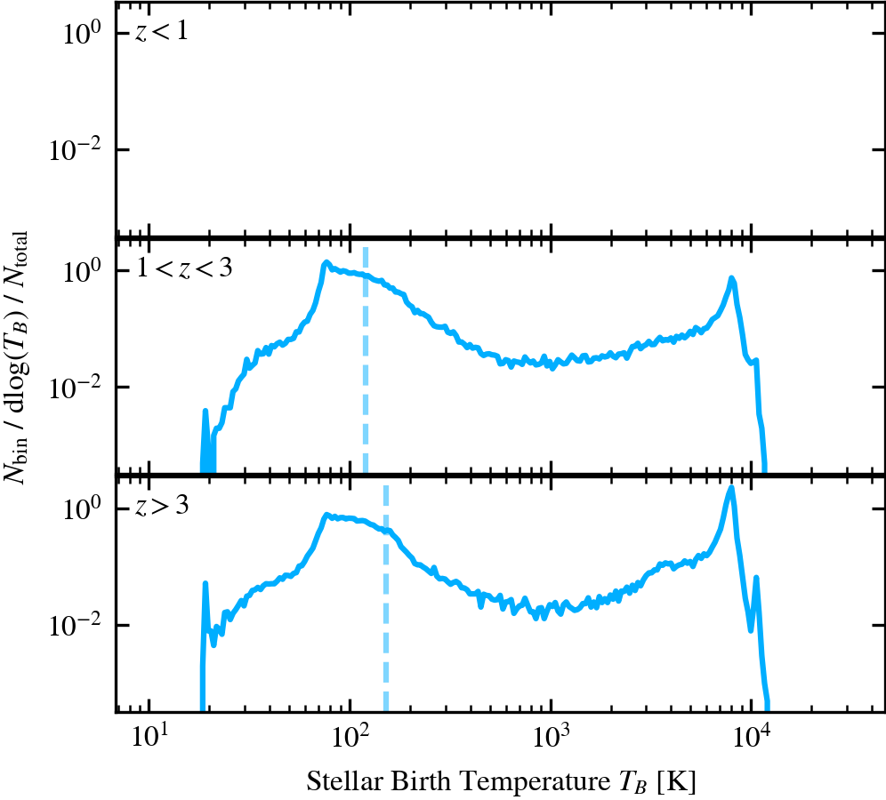
Stellar Birth Temperatures
Distributions of stellar birth temperatures, split by redshift. The y axis shows the number of stars per bin divided by the bin width and by the total number of stars. The dashed vertical lines show the median stellar birth-temperatures.
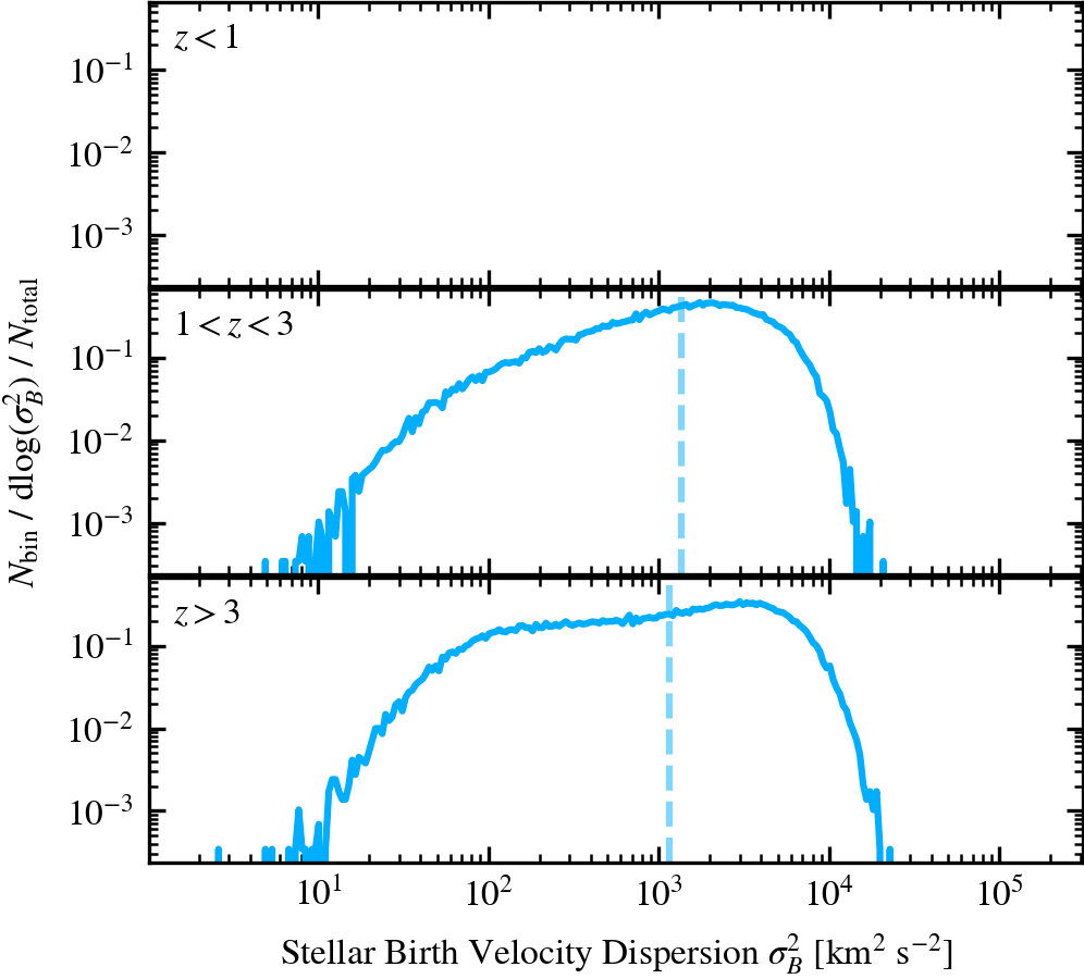
Stellar Birth Velocity Dispersions
Distributions of stellar birth velocity dispersions, split by redshift. The y axis shows the number of stars per bin divided by the bin width and by the total number of stars. The dashed vertical lines show the median stellar birth velocity dispersions.
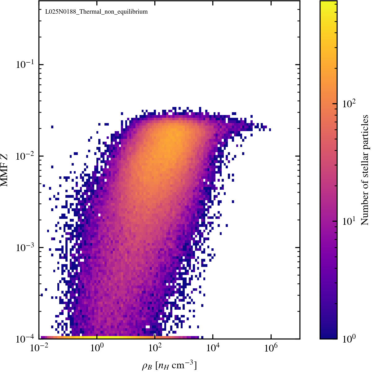
Stellar Birth Densities-Metallicity
Stellar birth densities vs metallicity diagram. The pixel colour indicates the number of stellar particles in the pixel. At a given birth density, particles with metallicities lower than the smallest value along the Y axis are placed in the lowest-metallicity bin. MMF stands for metal mass fraction.
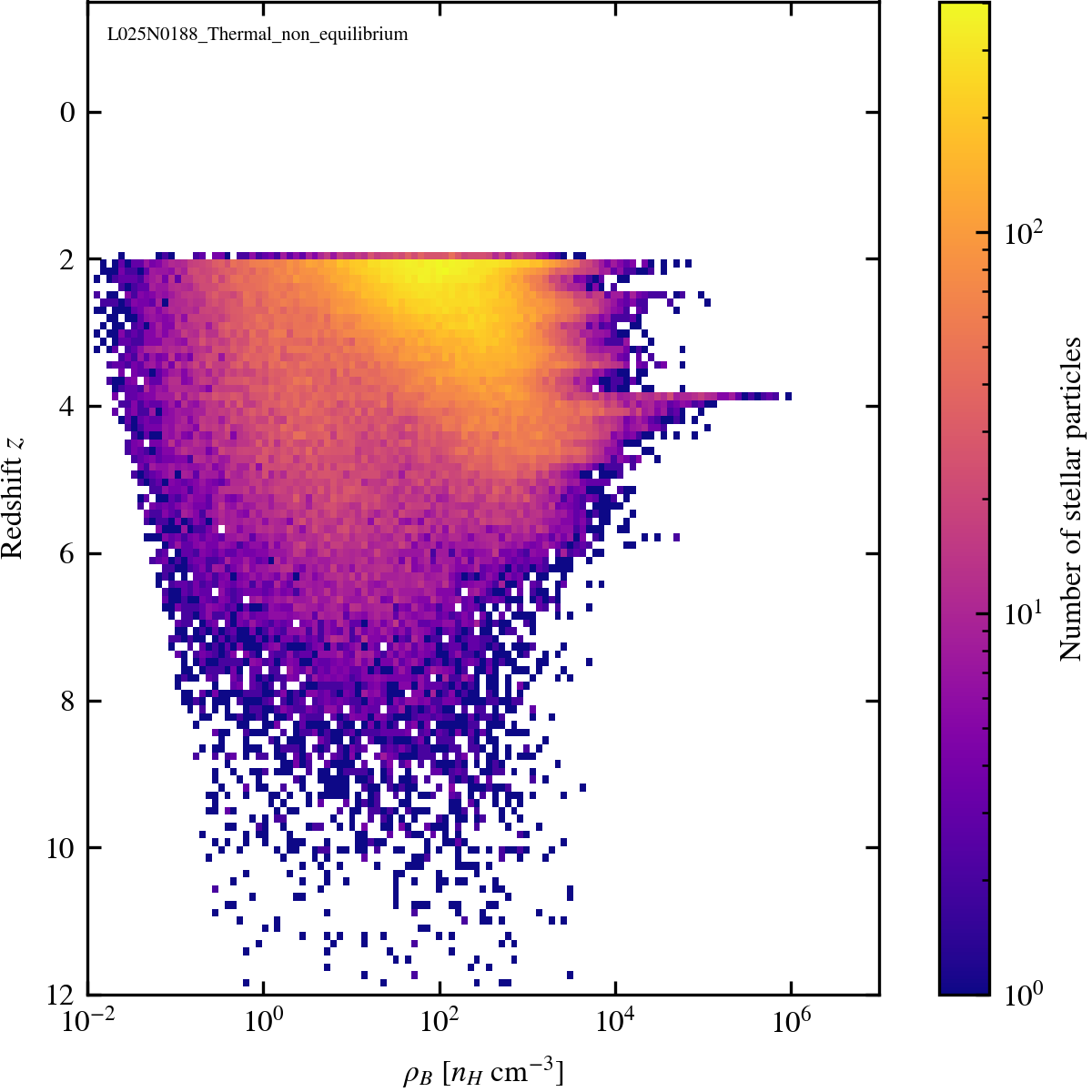
Stellar Birth Densities-Birth Redshift
Stellar birth densities vs birth redshift diagram. The pixel colour indicates the number of stellar particles in the pixel.
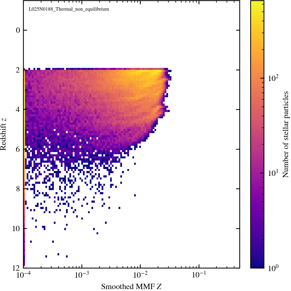
Stellar Metallicity-Birth Redshift
Stellar metallicity vs birth redshift diagram. The pixel colour indicates the number of stellar particles in the pixel. At a given birth redshift, particles with metallicities lower than the smallest value along the X axis are placed in the lowest-metallicity bin.
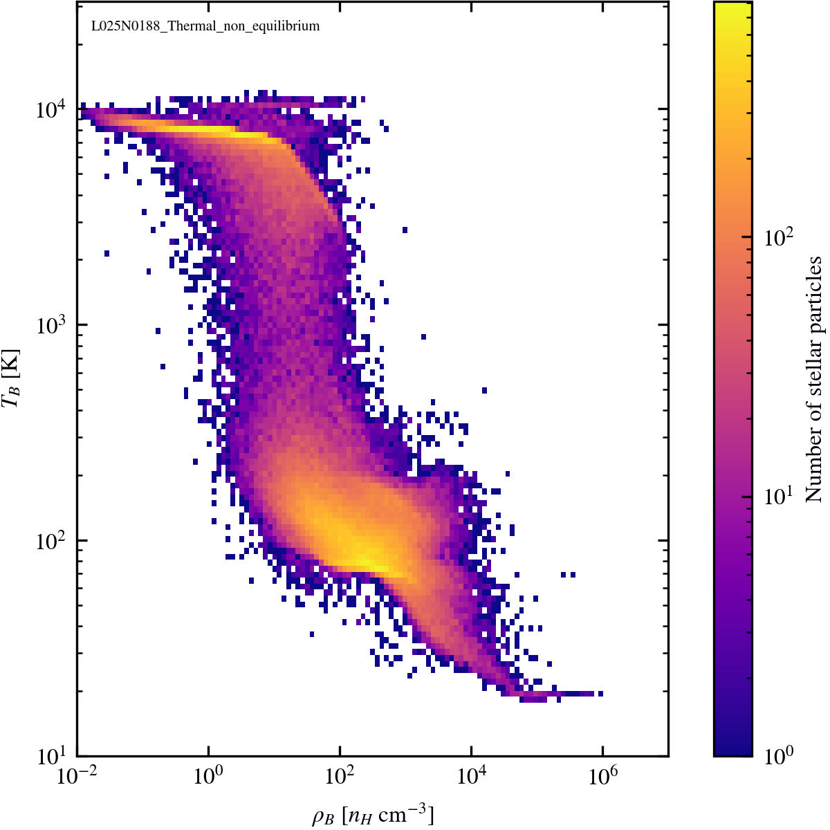
Stellar Birth Densities-Stellar Birth Temperatures
Stellar birth densities vs Stellar birth temperature diagram. The pixel colour indicates the number of stellar particles in the pixel.
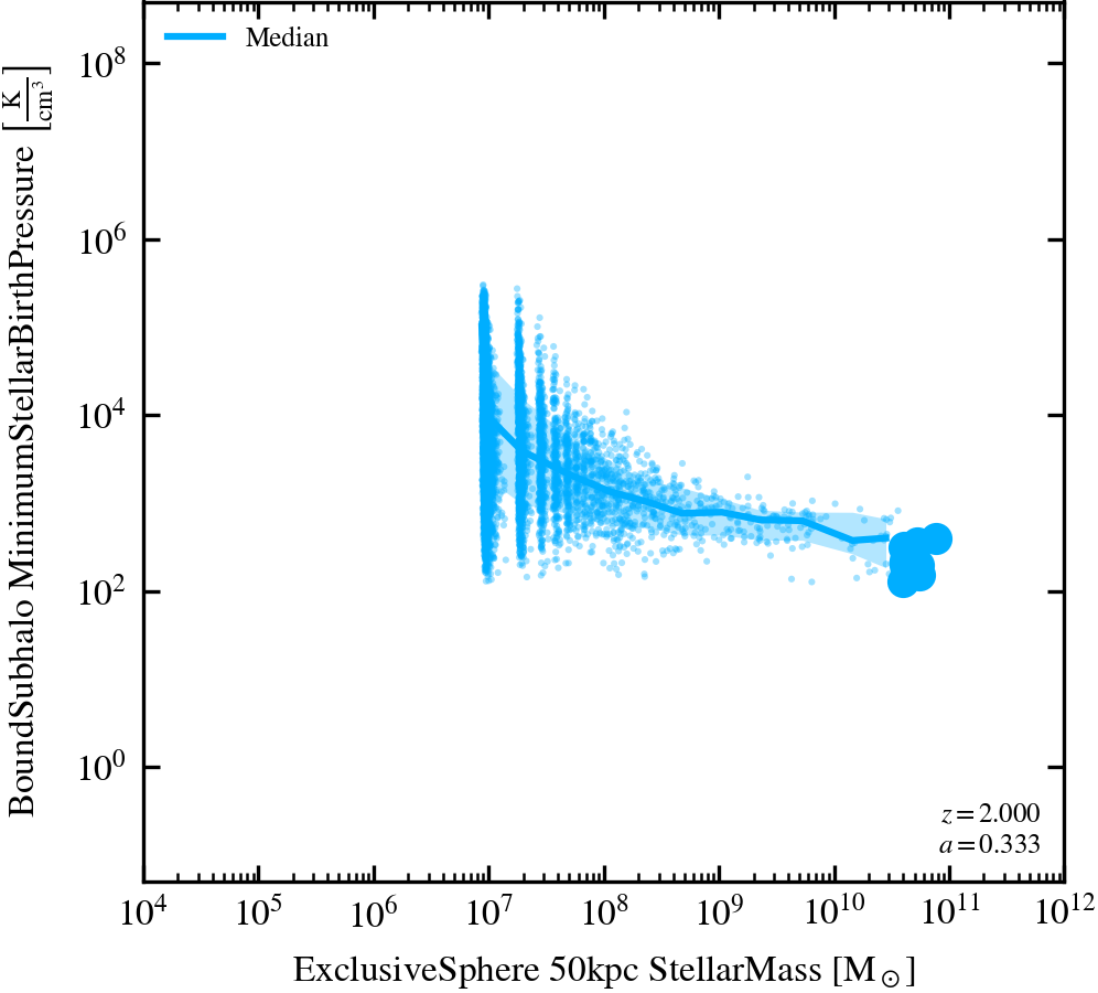
Minimal Stellar Birth Pressure-Stellar Mass relation
Includes all haloes, including subhaloes.
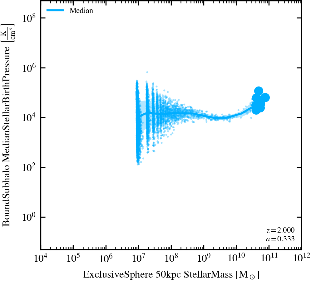
Median Stellar Birth Pressure-Stellar Mass relation
Includes all haloes, including subhaloes. The median is calculated based on the entire set of stellar particles within each (sub)halo.
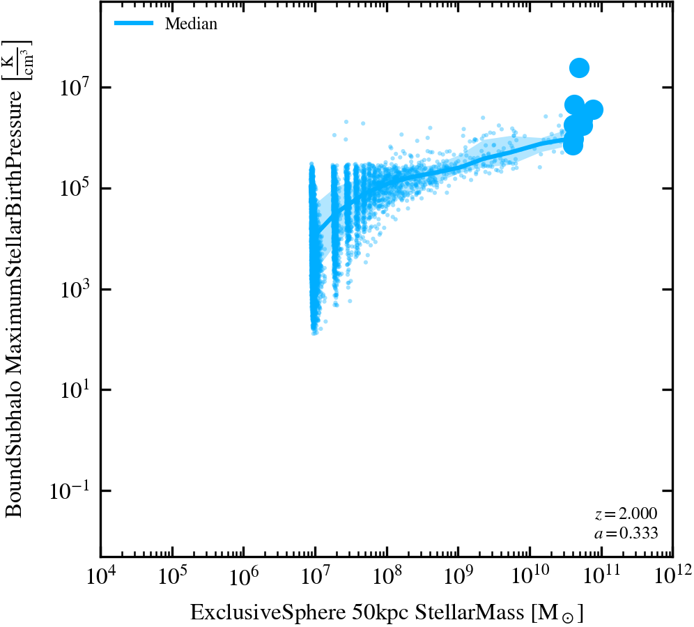
Maximal Stellar Birth Pressure-Stellar Mass relation
Includes all haloes, including subhaloes.
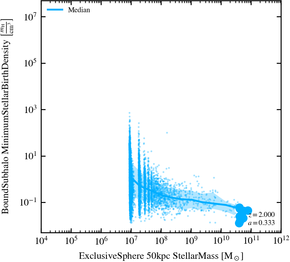
Minimal Stellar Birth Density-Stellar Mass relation
Includes all haloes, including subhaloes.
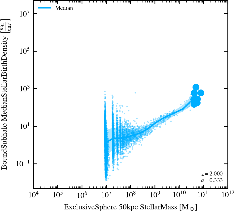
Median Stellar Birth Density-Stellar Mass relation
Includes all haloes, including subhaloes. The median is calculated based on the entire set of stellar particles within each (sub)halo.
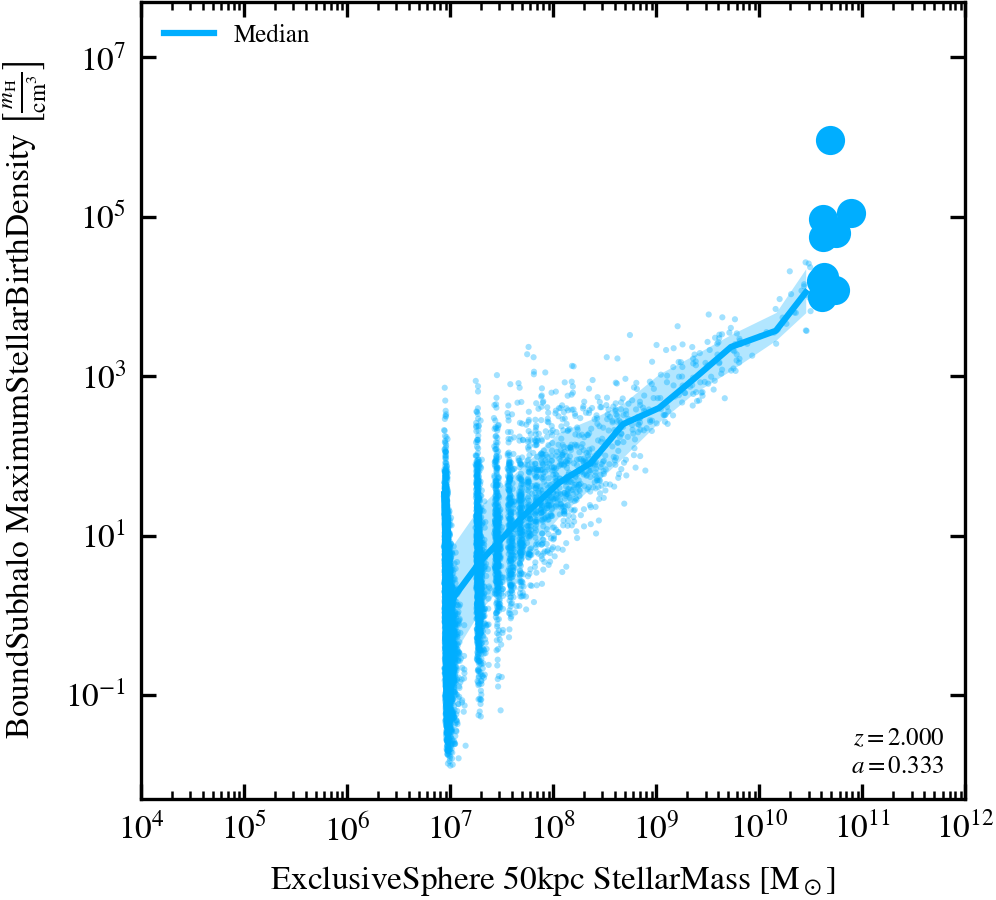
Maximal Stellar Birth Density-Stellar Mass relation
Includes all haloes, including subhaloes.
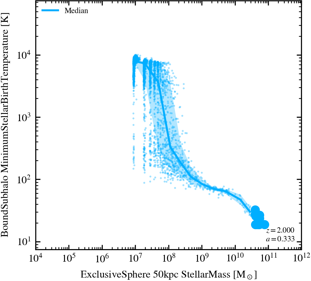
Minimal Stellar Birth Temperature-Stellar Mass relation
Includes all haloes, including subhaloes.
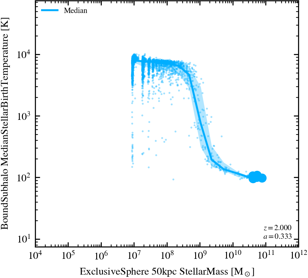
Median Stellar Birth Temperature-Stellar Mass relation
Includes all haloes, including subhaloes. The median is calculated based on the entire set of stellar particles within each (sub)halo.
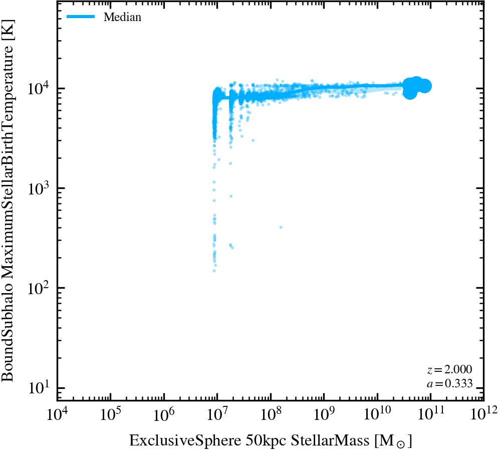
Maximal Stellar Birth Temperature-Stellar Mass relation
Includes all haloes, including subhaloes.
Stellar Mass Function
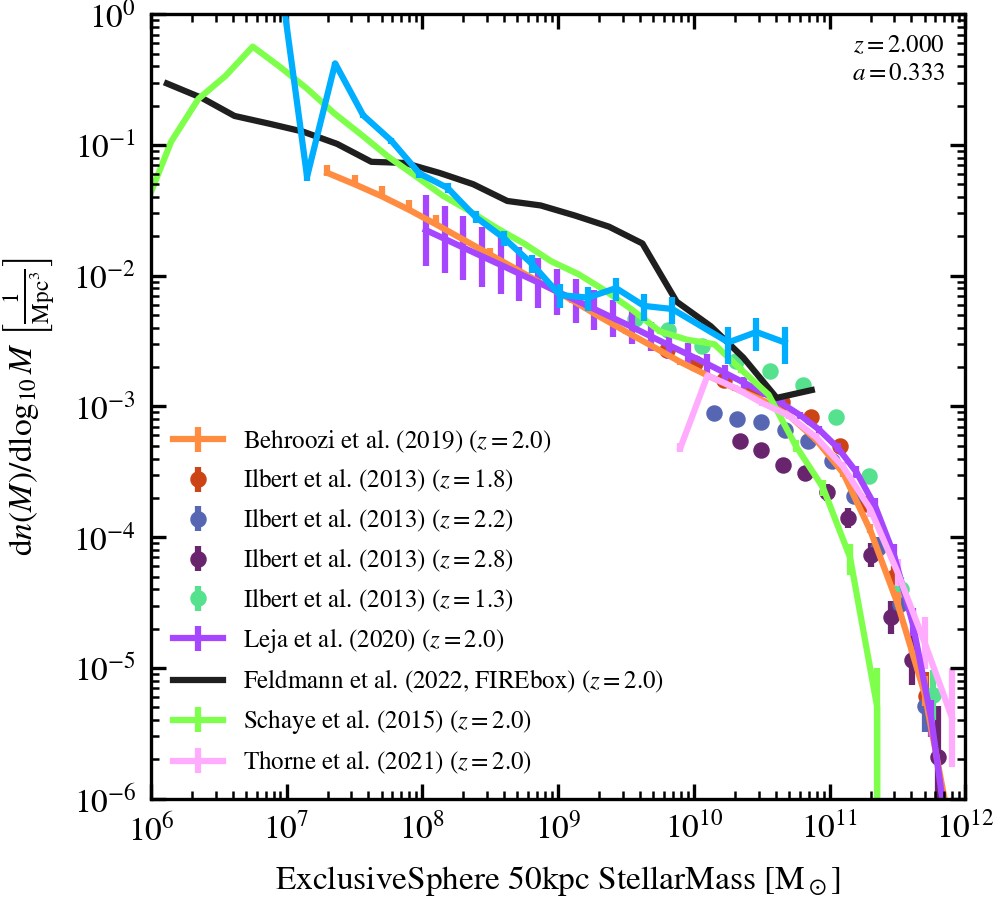
Stellar Mass Function (50 kpc aperture)
50 kpc aperture GSMF, showing all galaxies with a fixed bin-width of 0.2 dex.
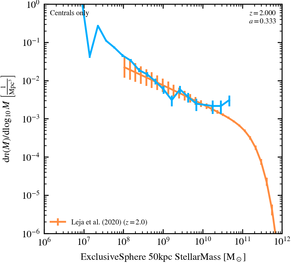
Stellar Mass Function (50 kpc aperture, centrals only)
50 kpc aperture GSMF, showing central galaxies only, with a fixed bin-width of 0.2 dex.
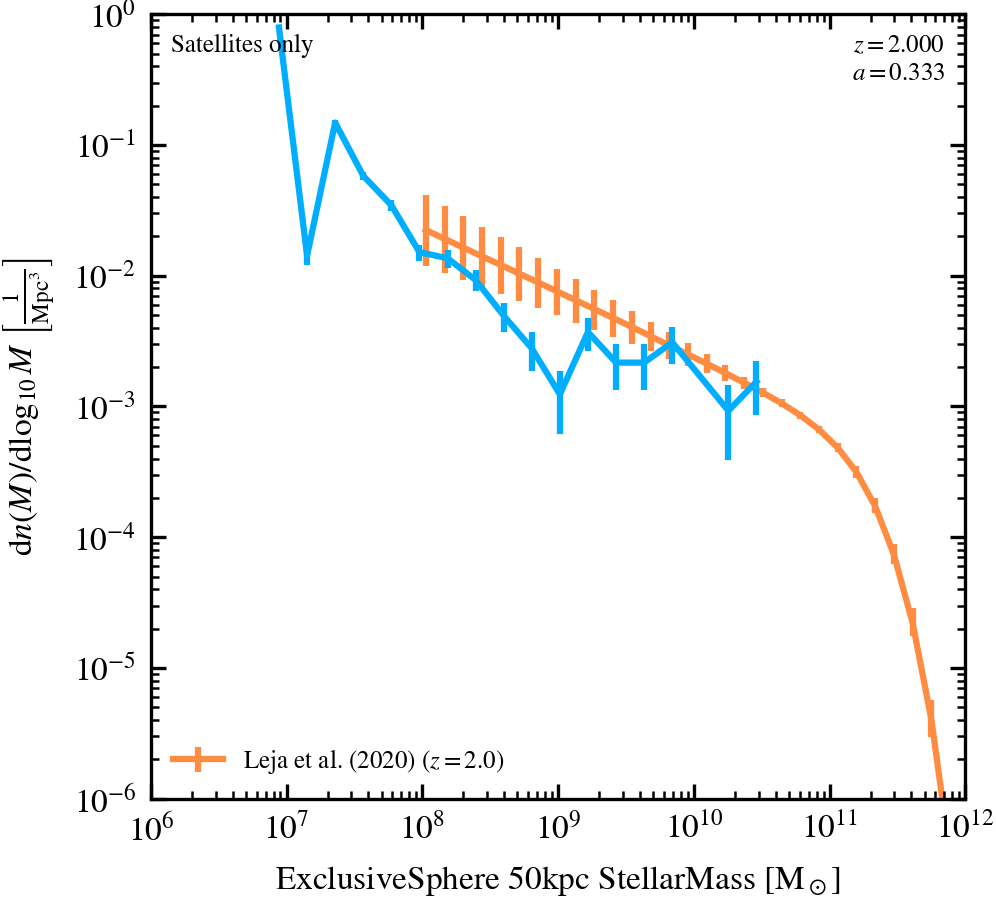
Stellar Mass Function (50 kpc aperture, satellites only)
50 kpc aperture GSMF, showing satellite galaxies only, with a fixed bin-width of 0.2 dex.
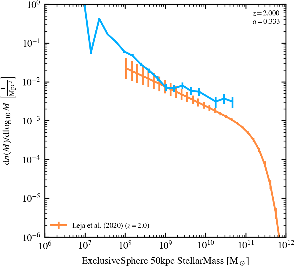
Stellar Mass Function (50 kpc aperture)
50 kpc aperture GSMF, showing all galaxies with a fixed bin-width of 0.2 dex. Only Leja et al. (2020) and Driver et al. (2021) data are shown.
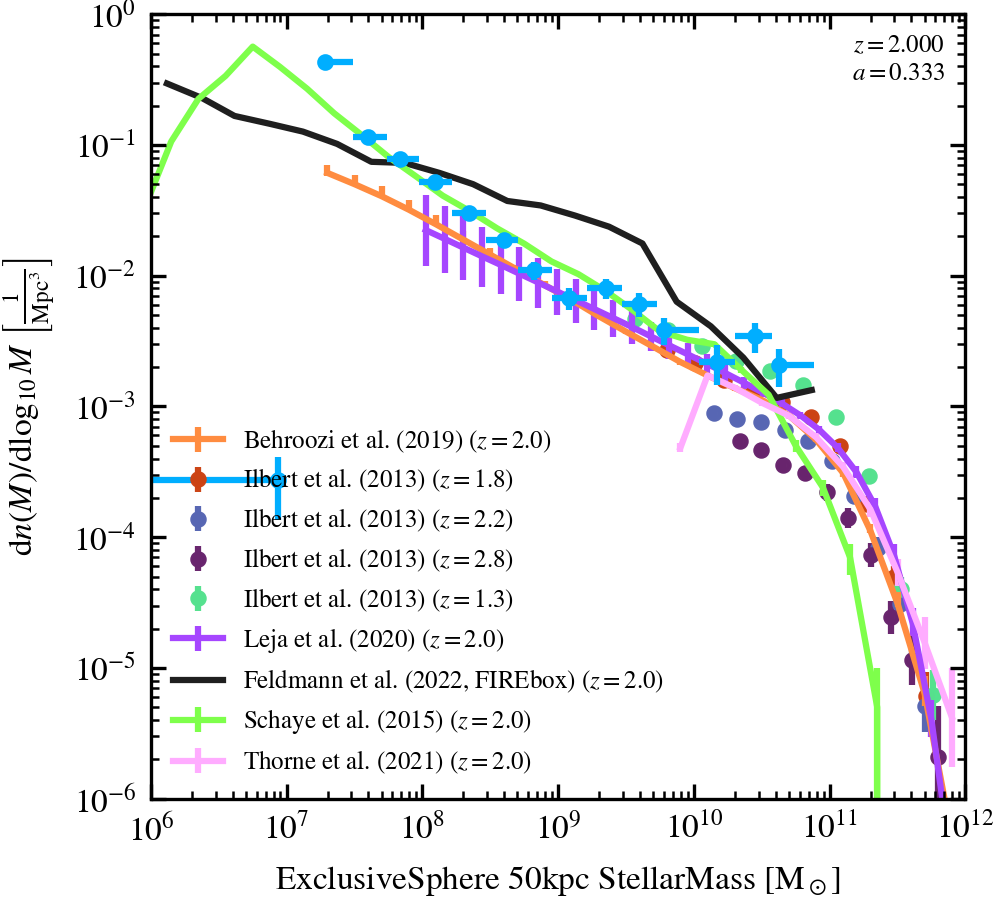
Stellar Mass Function (50 kpc aperture, adaptive)
50 kpc aperture GSMF, showing all galaxies with an adaptive bin-width.
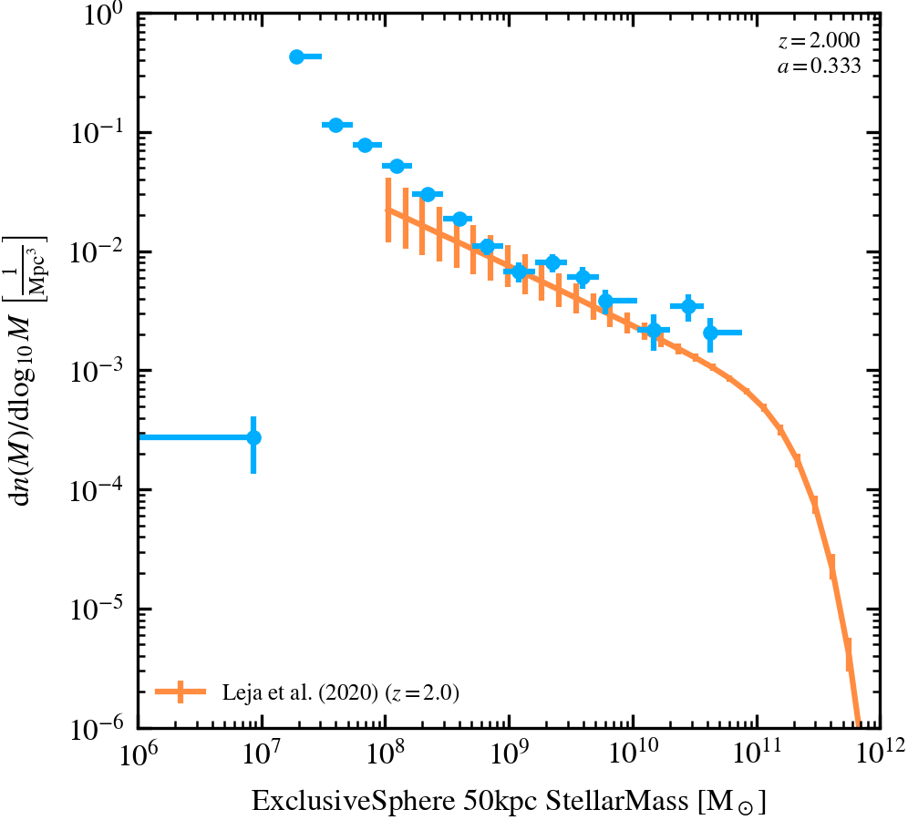
Stellar Mass Function (50 kpc aperture, adaptive)
50 kpc aperture GSMF, showing all galaxies with an adaptive bin-width. Only Leja et al. (2020) and Driver et al. (2021) data are shown.
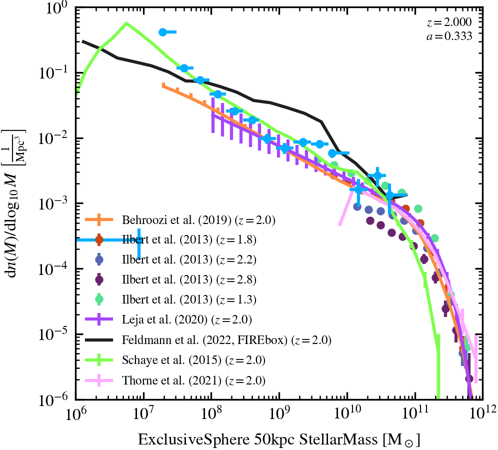
Stellar Mass Function (50 kpc aperture, adaptive, 25->50 Mpc box size correction)
50 kpc aperture GSMF, showing all galaxies with an adaptive bin-width. The data have been corrected to a box size of 50 Mpc, assuming the original simulation used a 25 Mpc box.
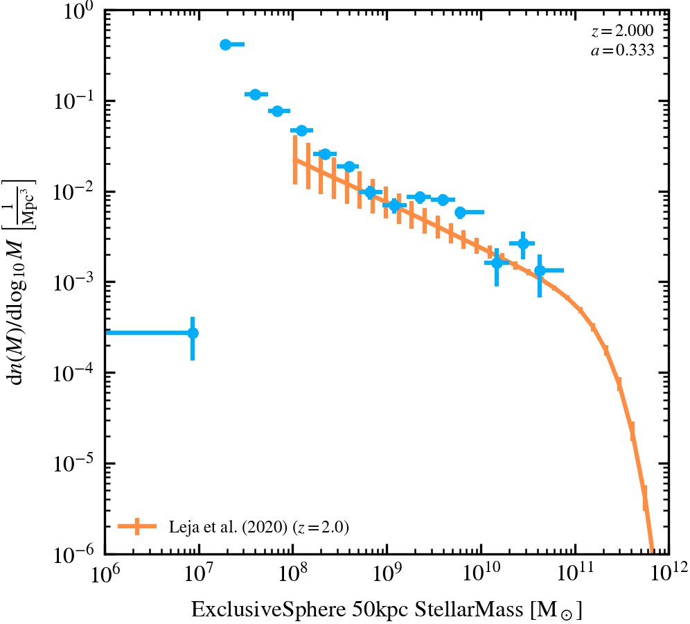
Stellar Mass Function (50 kpc aperture, adaptive, 25->50 Mpc box size correction)
50 kpc aperture GSMF, showing all galaxies with an adaptive bin-width. The data have been corrected to a box size of 50 Mpc, assuming the original simulation used a 25 Mpc box. Only Leja et al. (2020) and Driver et al. (2021) data are shown.
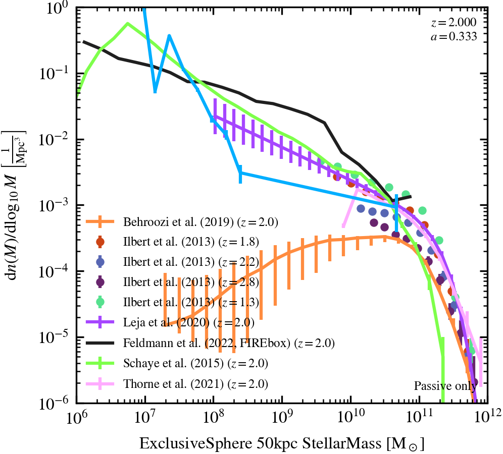
Stellar Mass Function (50 kpc aperture)
Only for passive galaxies, using an adaptive bin width.
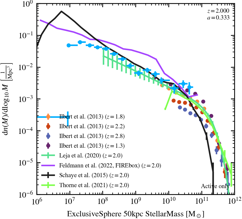
Stellar Mass Function (50 kpc aperture)
Only for active galaxies, using an adaptive bin width.
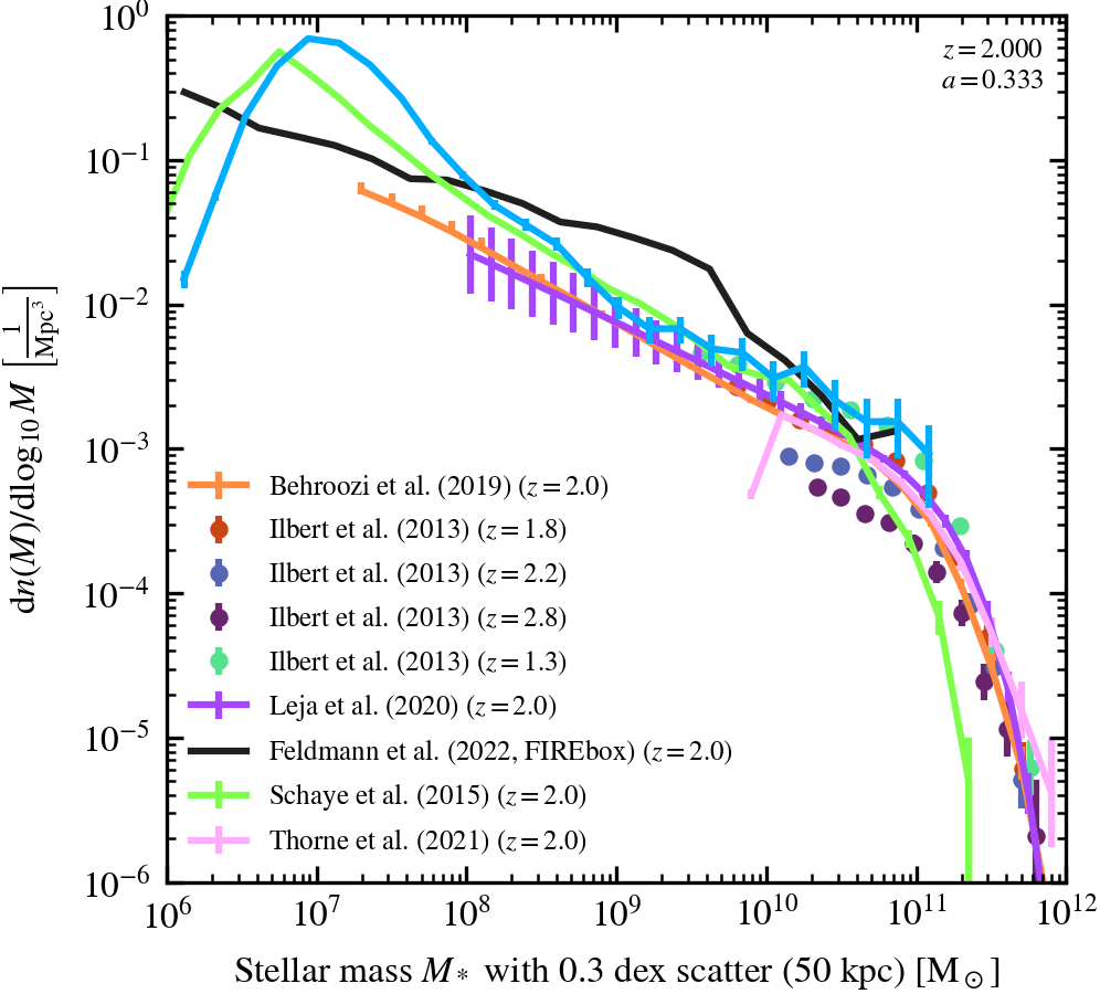
Stellar Mass Function (50 kpc aperture, with scatter)
50 kpc aperture GSMF, showing all galaxies with a fixed bin-width of 0.2 dex, with an additional 0.3 dex log-normal scatter in the stellar mass.
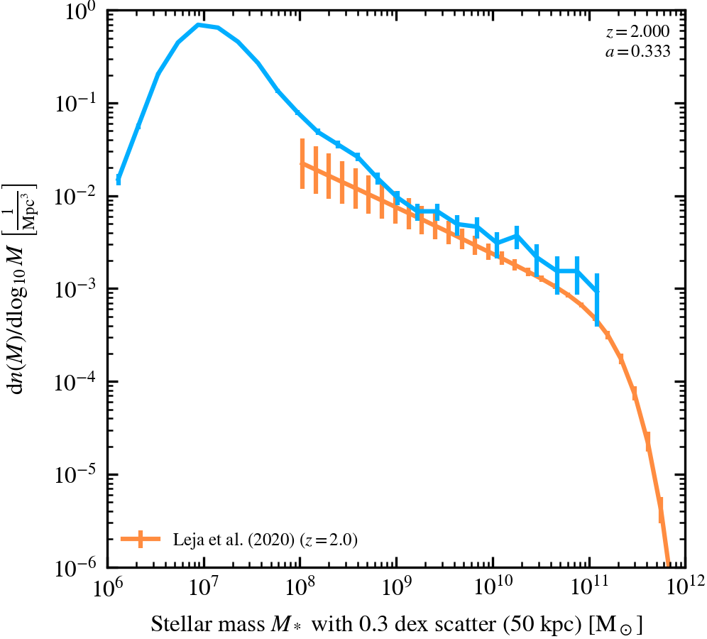
Stellar Mass Function (50 kpc aperture, with scatter)
50 kpc aperture GSMF, showing all galaxies with a fixed bin-width of 0.2 dex, with an additional 0.3 dex log-normal scatter in the stellar mass. Only Leja et al. (2020) and Driver et al. (2021) data are shown.
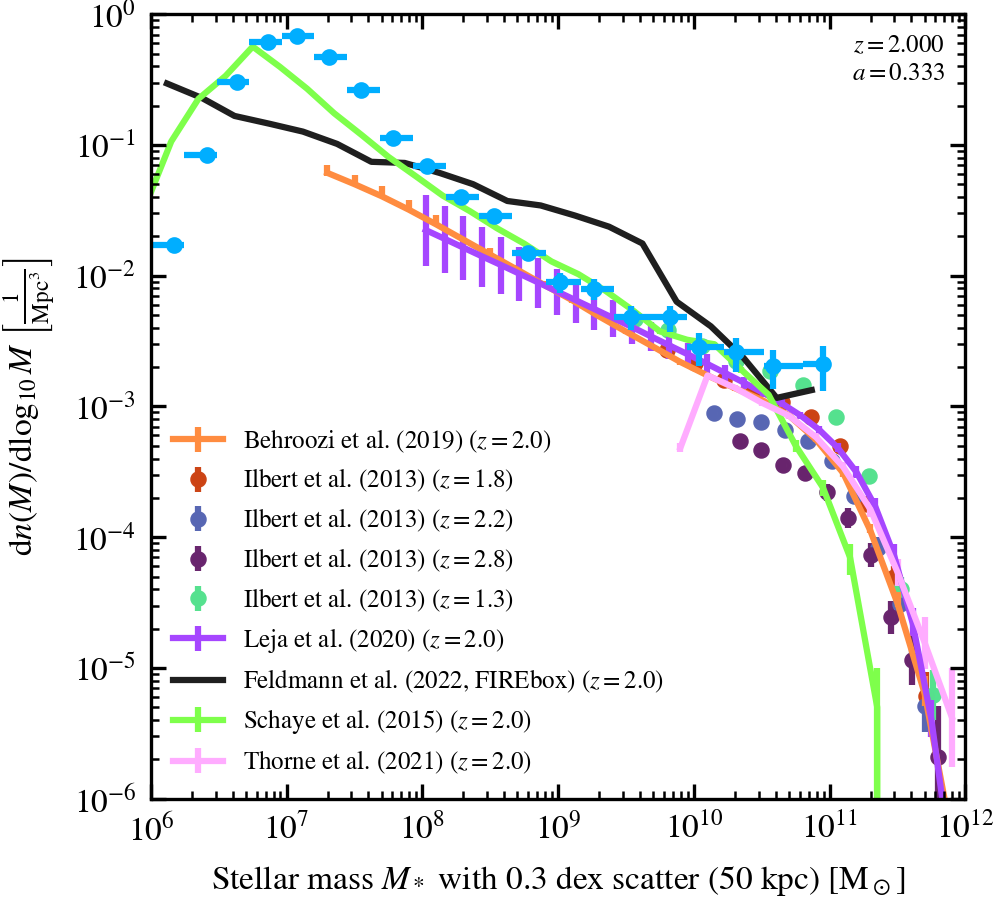
Stellar Mass Function (50 kpc aperture, adaptive, with scatter)
50 kpc aperture GSMF, showing all galaxies with an adaptive bin-width, with an additional 0.3 dex log-normal scatter in the stellar mass.
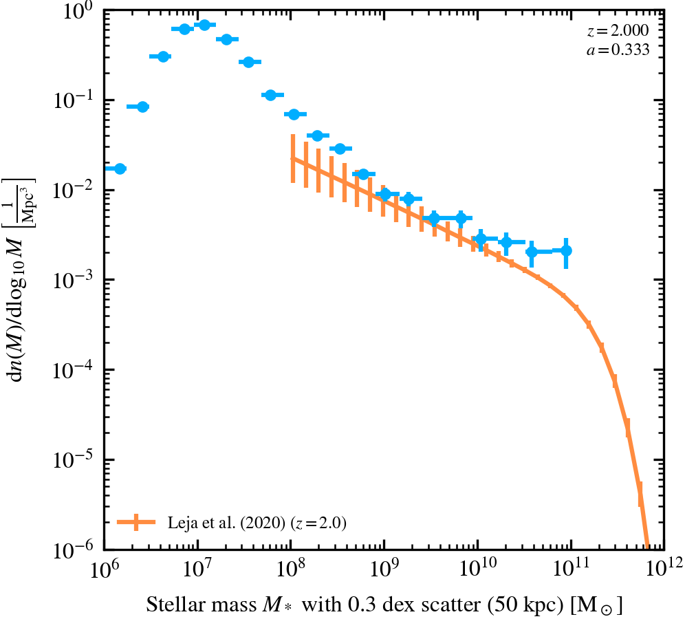
Stellar Mass Function (50 kpc aperture, adaptive, with scatter)
50 kpc aperture GSMF, showing all galaxies with an adaptive bin-width, with an additional 0.3 dex log-normal scatter in the stellar mass. Only Leja et al. (2020) and Driver et al. (2021) data are shown.
Stellar Mass-Halo Mass
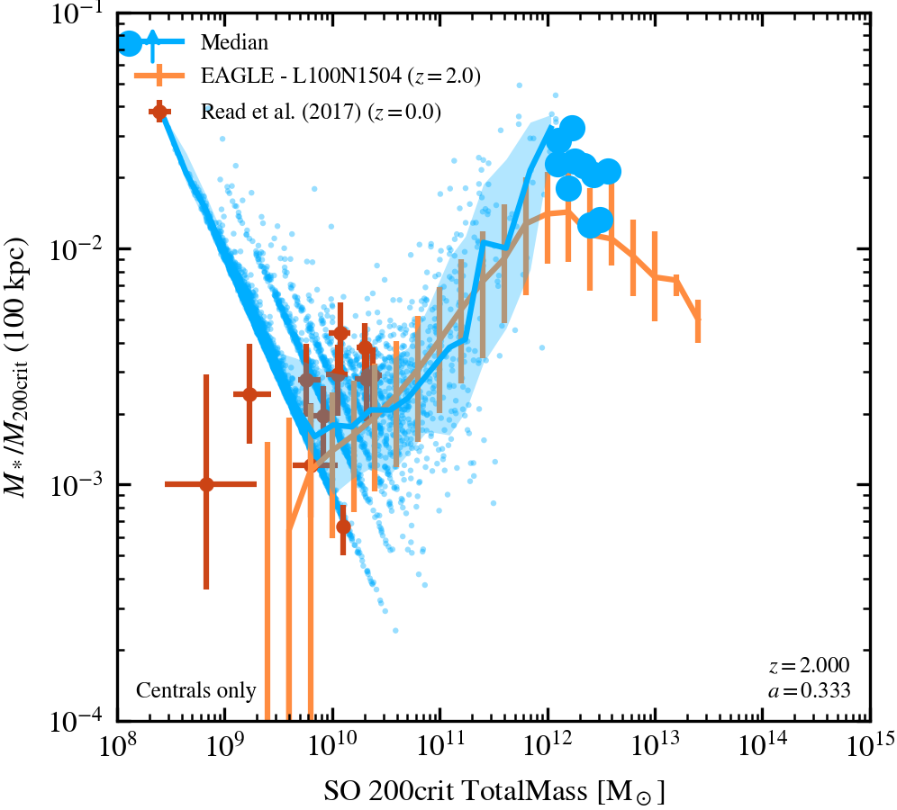
Stellar Mass-Halo Mass relation (ratio, 100 kpc aperture, $M_{200,crit}$, centrals only)
Includes only central haloes.
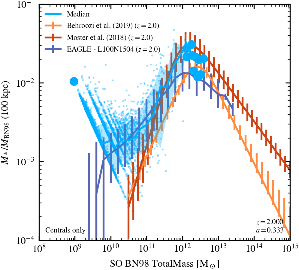
Stellar Mass-Halo Mass relation (ratio, 100 kpc aperture, $M_{\rm BN98}$, centrals only)
Includes only central haloes.
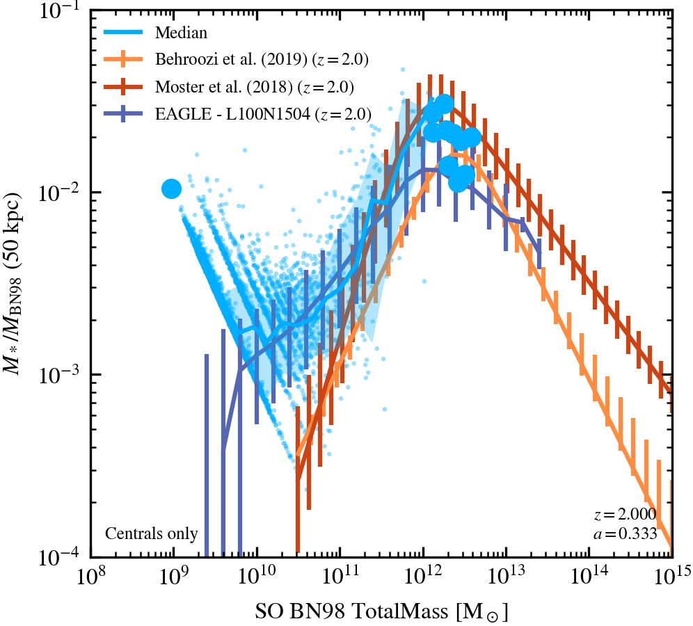
Stellar Mass-Halo Mass relation (ratio, 50 kpc aperture, $M_{\rm BN98}$, centrals only)
Includes only central haloes.
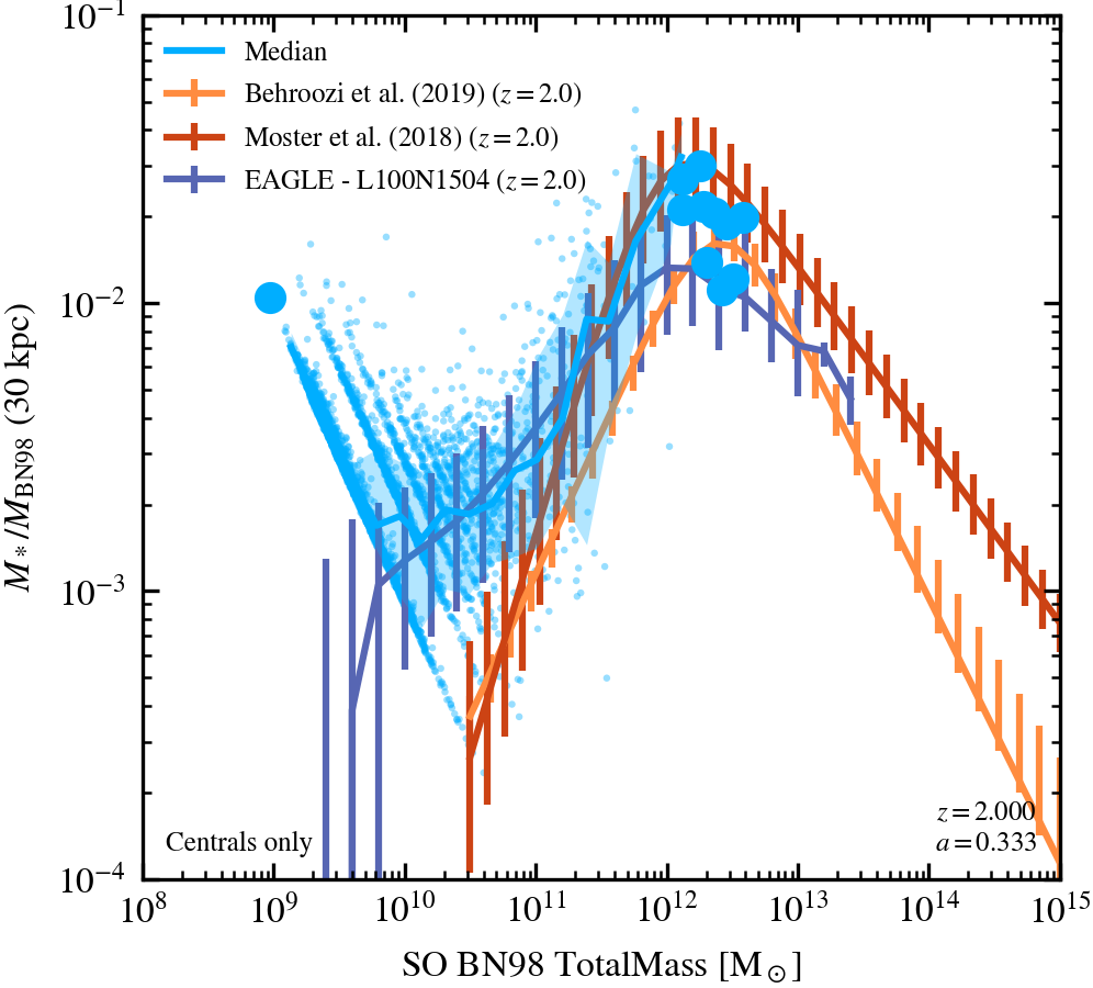
Stellar Mass-Halo Mass relation (ratio, 30 kpc aperture, $M_{\rm BN98}$, centrals only)
Includes only central haloes.
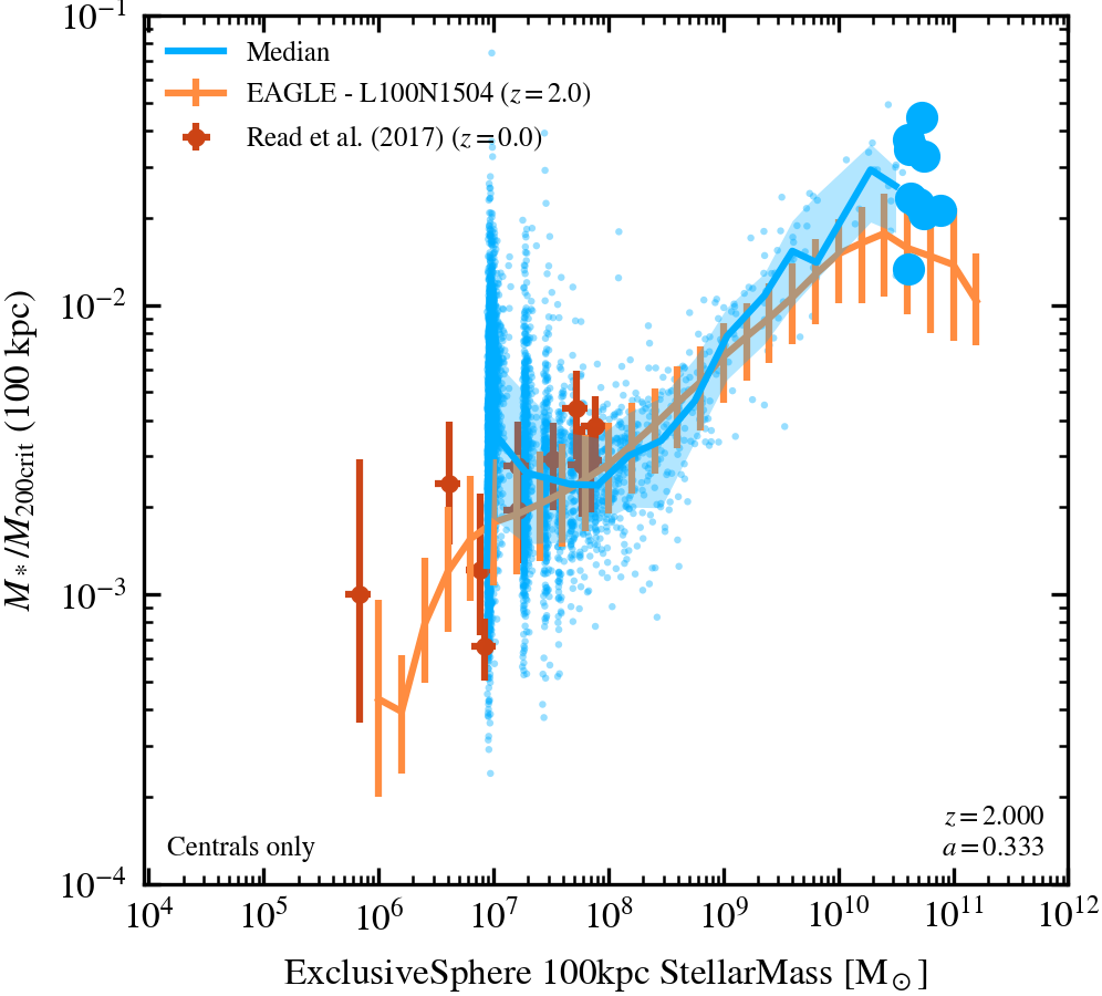
Stellar Mass-Halo Mass relation (ratio, 100 kpc aperture, $M_{200,crit}$, centrals only, stellar x-axis)
Includes only central haloes.
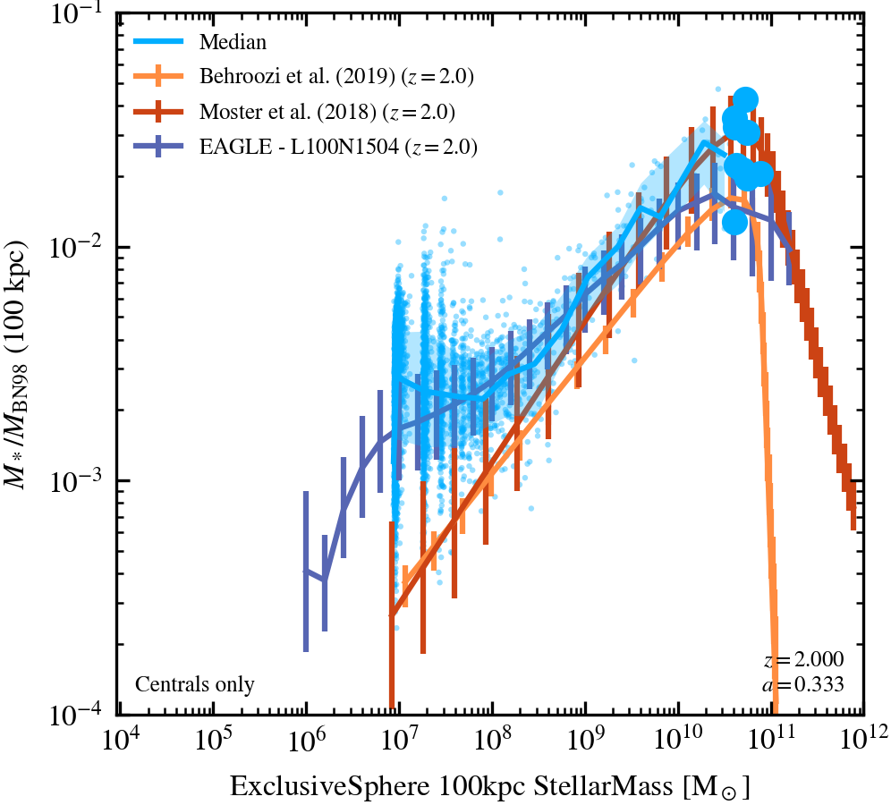
Stellar Mass-Halo Mass relation (ratio, 100 kpc aperture, $M_{\rm BN98}$, centrals only, stellar x-axis)
Includes only central haloes.
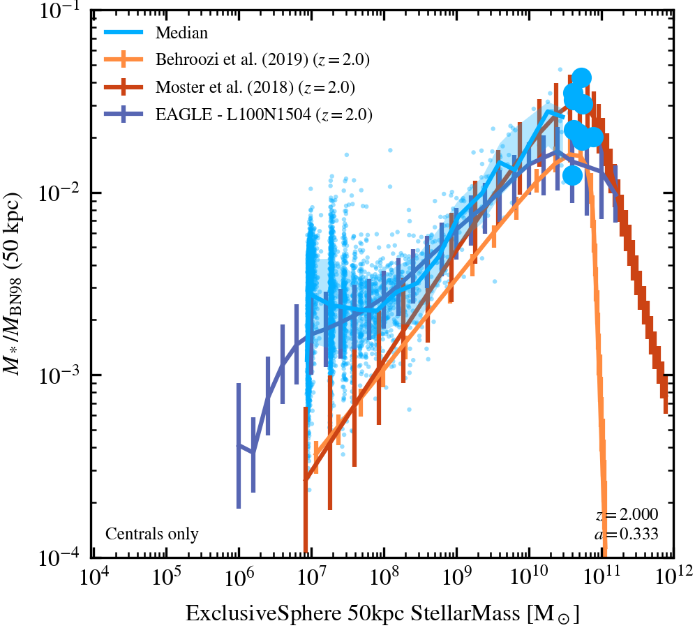
Stellar Mass-Halo Mass relation (ratio, 50 kpc aperture, $M_{\rm BN98}$, centrals only, stellar x-axis)
Includes only central haloes.
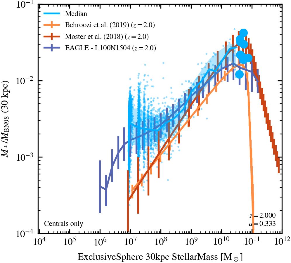
Stellar Mass-Halo Mass relation (ratio, 30 kpc aperture, $M_{\rm BN98}$, centrals only, stellar x-axis)
Includes only central haloes.
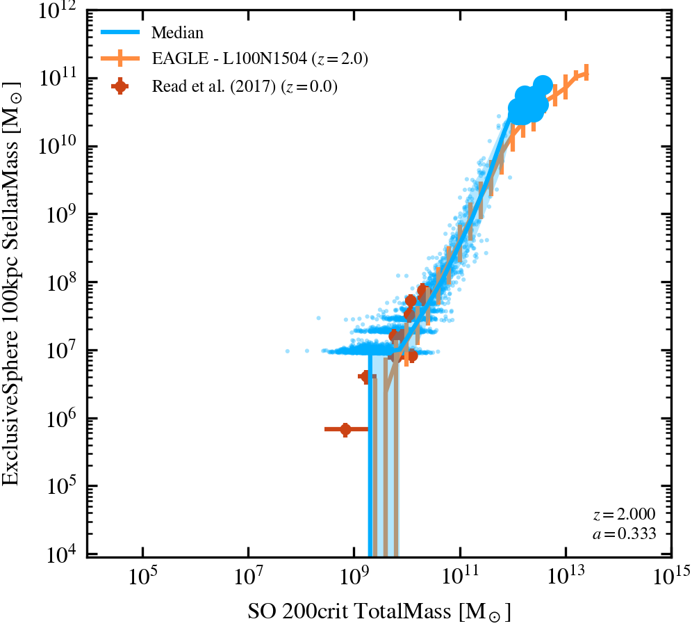
Stellar Mass-Halo Mass relation (100 kpc aperture, $M_{200,crit}$)
Includes all haloes, including subhaloes.
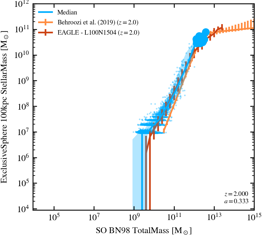
Stellar Mass-Halo Mass relation (100 kpc aperture, $M_{\rm BN98}$)
Includes all haloes, including subhaloes.
Stellar Mass-Halo Mass (BCGs)
Stellar Mass-Halo Mass relation (10 kpc 2D aperture, $M_{200,crit}$, centrals only)
Includes only central haloes, and excludes the contribution of satellites in projection, for both the simulated and observed data. The halo masses in observations by DeMaio et al. (2020) and the semi-empirical model by Huang et al. (2022) were converted from the $M_{500}$ and $M_\mathrm{BN98}$ definitions, respectively, to a $M_{200}$ definition (critical overdensity), by assuming an NFW profile and concentration $c=5$. The halo masses from Golden-Marx et al. (2022) were converted from a mean overdensity to critical overdensity (factor 200) definition. None of the halo masses are corrected for (hydrostatic and other) bias. The IMF from observations by Golden-Marx et al. (2022) was converted from Salpeter to Chabrier. Cosmology corrections were not needed. The data that are of intermediate-redshift objects can be used for comparison here because the evolution of BCG stellar cores is observed to be negligible in this regime. The Huang et al. (2022) model is tailored to groups and clusters, and uses aperture definitions for stellar masses, not only for its predictions but also for the observational data used for calibration.
Stellar Mass-Halo Mass relation (30 kpc 2D aperture, $M_{200,crit}$, centrals only)
Includes only central haloes, and excludes the contribution of satellites in projection, for both the simulated and observed data. The halo masses in observations by Kravstov et al. (2018) and the semi-empirical model by Huang et al. (2022) were converted from the $M_{500}$ and $M_\mathrm{BN98}$ definitions, respectively, to a $M_{200}$ definition (critical overdensity), by assuming an NFW profile and concentration $c=5$. The halo masses from Golden-Marx et al. (2022) were converted from a mean overdensity to critical overdensity (factor 200) definition. None of the halo masses are corrected for (hydrostatic and other) bias. The IMF from observations by Golden-Marx et al. (2022) was converted from Salpeter to Chabrier. Cosmology corrections were not needed. The data that are of intermediate-redshift objects can be used for comparison here because the evolution of BCG stellar cores is observed to be negligible in this regime. The Huang et al. (2022) model is tailored to groups and clusters, and uses aperture definitions for stellar masses, not only for its predictions but also for the observational data used for calibration.
Stellar Mass-Halo Mass relation (50 kpc 2D aperture, $M_{200,crit}$, centrals only)
Includes only central haloes, and excludes the contribution of satellites in projection, for both the simulated and observed data. The halo masses in observations by Gonzalez et al. (2013) and Kravstov et al. (2018), as well as the semi-empirical model by Huang et al. (2022), were converted from the $M_{500}$ and $M_\mathrm{BN98}$ definitions to a $M_{200}$ definition (critical overdensity), by assuming an NFW profile and concentration $c=5$. The halo masses from Golden-Marx et al. (2022) were converted from a mean overdensity to critical overdensity (factor 200) definition. None of the halo masses are corrected for (hydrostatic and other) bias. The IMF from observations by Golden-Marx et al. (2022) was converted from Salpeter to Chabrier. Cosmology corrections were not needed. The data that are of intermediate-redshift objects can may be a slight underestimate due to weak growth of the ICL with redshift. The Huang et al. (2022) model is tailored to groups and clusters, and uses aperture definitions for stellar masses, not only for its predictions but also for the observational data used for calibration.
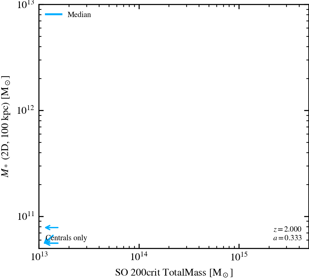
Stellar Mass-Halo Mass relation (100 kpc 2D aperture, $M_{200,crit}$, centrals only)
Includes only central haloes, and excludes the contribution of satellites in projection, for both the simulated and observed data. The halo masses in observations by Kravstov et al. (2018) and DeMaio et al. (2020), as well as the semi-empirical model by Huang et al. (2022), were converted from the $M_{500}$ and $M_\mathrm{BN98}$ definitions to a $M_{200}$ definition (using the critical overdensity), by assuming an NFW profile and concentration $c=5$. The halo masses from Golden-Marx et al. (2022) were converted from a mean overdensity to critical overdensity (factor 200) definition. None of the halo masses are corrected for (hydrostatic and other) bias. The IMF from observations by Golden-Marx et al. (2022) was converted from Salpeter to Chabrier. Cosmology corrections were not needed. The data that are of intermediate-redshift objects are likely a slight underestimate due to weak growth of the ICL with redshift. The Huang et al. (2022) model is tailored to groups and clusters, and uses aperture definitions for stellar masses, not only for its predictions but also for the observational data used for calibration.
Stellar Metal Abundances
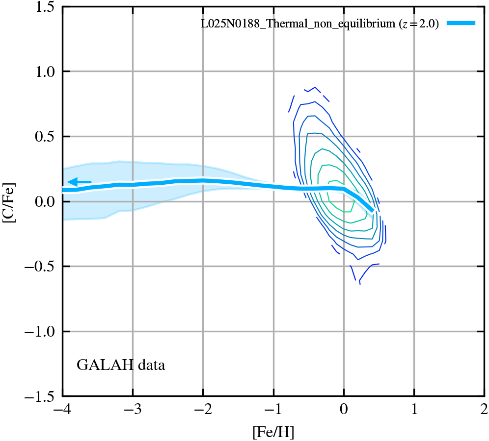
[Fe/H] vs [C/Fe]
[Fe/H] vs [C/Fe] using Asplund et al. (2009) values for [Fe/H]Sun = 7.5 and [C/H]Sun = 8.43. The median [C/Fe] vs median [Fe/H] is indicated by the solid curve(s). The scatter points show abundances of individual stellar particles. The observational data for MW compiles the data from the GALAH survey (Buder et al. 2021). Contours use a log scale with 0.04 bin size and a minimum star count of 10. All recommended flags are applied to GALAH data to select stars (SN, FE/H and X/Fe quality flags). The arrows at [Fe/H]=-4 indicate the median value of [C/Fe] of gas with [Fe/H]<-4.
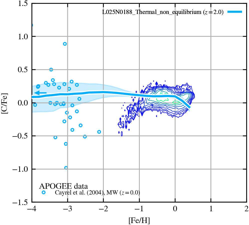
[Fe/H] vs [C/Fe]
[Fe/H] vs [C/Fe] using Asplund et al. (2009) values for [Fe/H]Sun = 7.5 and [C/H]Sun = 8.43. The median [C/Fe] vs median [Fe/H] is indicated by the solid curve(s). The scatter points show abundances of individual stellar particles. The observational data for MW compiles the data from the APOGEE survey (Holtzman et al. 2018) and AstroNN added-value catalog (Leung, H.W. & Bovy, Jo 2019b). We create 6 stellar distributions by selecting stars from APOGEE based on galactocentric radial & azimuthal cuts, and combine them in order to derive a joint stellar abundance distribution that gives less weight to stars in the solar vicinity. The resulting contours use a log scale with 0.2 bin size. The arrows at [Fe/H]=-4 indicate the median value of [C/Fe] of gas with [Fe/H]<-4.
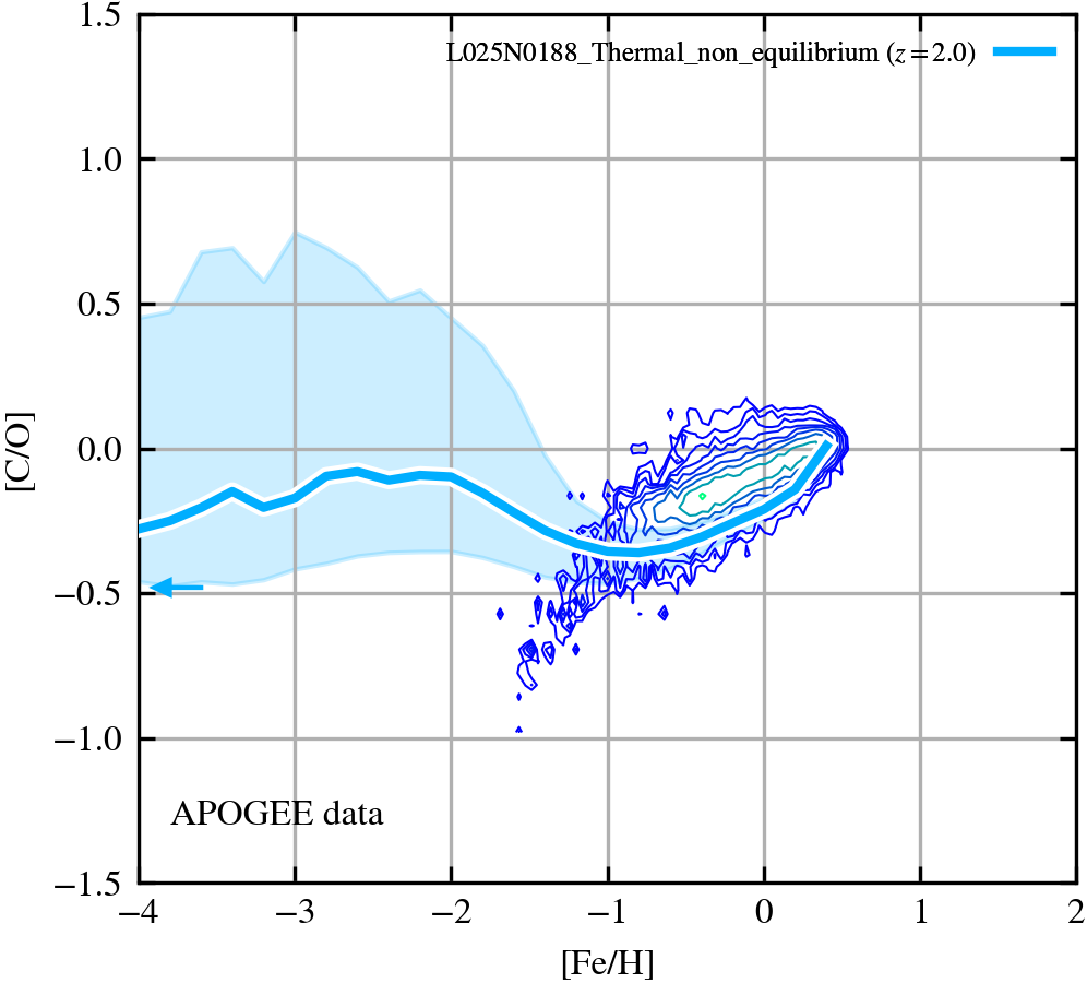
[Fe/H] vs [C/O]
[Fe/H] vs [C/O] using Asplund et al. (2009) values for [O/H]Sun = 8.69 and [C/H]Sun = 8.43. The median [C/O] vs median [Fe/H] is indicated by the solid curve(s). The scatter points show abundances of individual stellar particles. The observational data for MW compiles the data from the APOGEE survey (Holtzman et al. 2018) and AstroNN added-value catalog (Leung, H.W. & Bovy, Jo 2019b). We create 6 stellar distributions by selecting stars from APOGEE based on galactocentric radial & azimuthal cuts, and combine them in order to derive a joint stellar abundance distribution that gives less weight to stars in the solar vicinity. The resulting contours use a log scale with 0.2 bin size. The arrows at [Fe/H]=-4 indicate the median value of [C/O] of gas with [Fe/H]<-4.
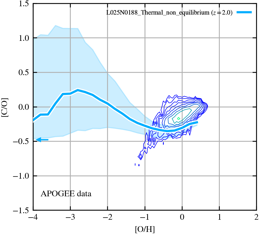
[O/H] vs [C/O]
[O/H] vs [C/O] using Asplund et al. (2009) values for [O/H]Sun = 8.69 and [C/H]Sun = 8.43. The median [C/O] vs median [O/H] is indicated by the solid curve(s). The scatter points show abundances of individual stellar particles. The observational data for MW compiles the data from the APOGEE survey (Holtzman et al. 2018) and AstroNN added-value catalog (Leung, H.W. & Bovy, Jo 2019b). We create 6 stellar distributions by selecting stars from APOGEE based on galactocentric radial & azimuthal cuts, and combine them in order to derive a joint stellar abundance distribution that gives less weight to stars in the solar vicinity. The resulting contours use a log scale with 0.2 bin size. The arrows at [O/H]=-4 indicate the median value of [C/O] of gas with [O/H]<-4.
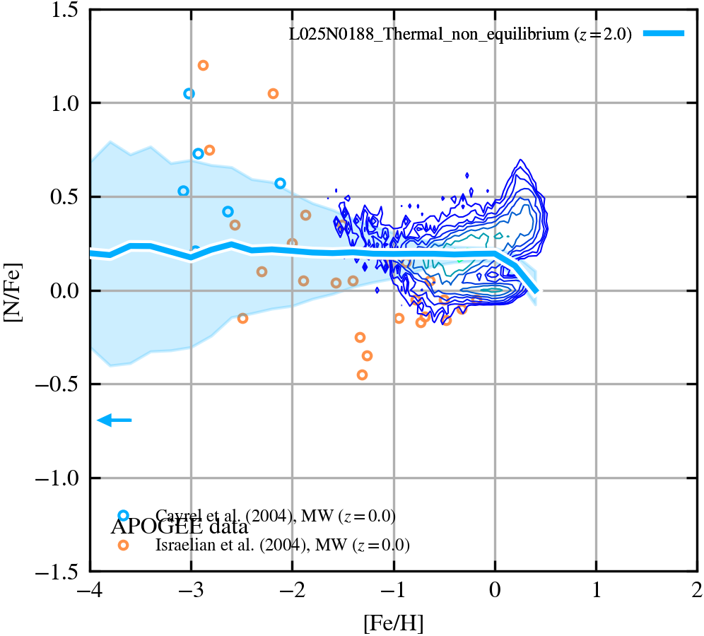
[Fe/H] vs [N/Fe]
[Fe/H] vs [N/Fe] using Asplund et al. (2009) values for [Fe/H]Sun = 7.5 and [N/H]Sun = 7.83. The median [N/Fe] vs median [Fe/H] is indicated by the solid curve(s). The scatter points show abundances of individual stellar particles. The observational data for MW compiles the data from the APOGEE survey (Holtzman et al. 2018) and AstroNN added-value catalog (Leung, H.W. & Bovy, Jo 2019b). We create 6 stellar distributions by selecting stars from APOGEE based on galactocentric radial & azimuthal cuts, and combine them in order to derive a joint stellar abundance distribution that gives less weight to stars in the solar vicinity. The resulting contours use a log scale with 0.2 bin size. The arrows at [Fe/H]=-4 indicate the median value of [N/Fe] of gas with [Fe/H]<-4.
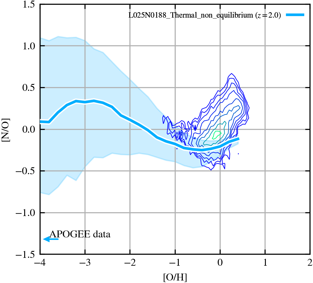
[O/H] vs [N/O]
[O/H] vs [N/O] using Asplund et al. (2009) values for [O/H]Sun = 8.69 and [N/H]Sun = 7.83. The median [N/O] vs median [O/H] is indicated by the solid curve(s). The scatter points show abundances of individual stellar particles. The observational data for MW compiles the data from the APOGEE survey (Holtzman et al. 2018) and AstroNN added-value catalog (Leung, H.W. & Bovy, Jo 2019b). We create 6 stellar distributions by selecting stars from APOGEE based on galactocentric radial & azimuthal cuts, and combine them in order to derive a joint stellar abundance distribution that gives less weight to stars in the solar vicinity. The resulting contours use a log scale with 0.2 bin size. The arrows at [O/H]=-4 indicate the median value of [N/O] of gas with [O/H]<-4.
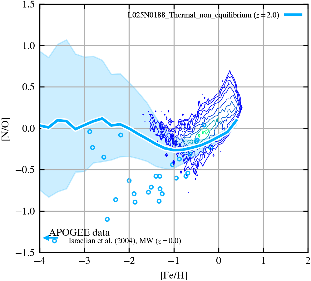
[Fe/H] vs [N/O]
[Fe/H] vs [N/O] using Asplund et al. (2009) values for [Fe/H]Sun = 7.5, [N/H]Sun = 7.83 and [O/H]Sun = 8.69. The median [N/O] vs median [Fe/H] is indicated by the solid curve(s). The scatter points show abundances of individual stellar particles. The observational data for MW compiles the data from the APOGEE survey (Holtzman et al. 2018) and AstroNN added-value catalog (Leung, H.W. & Bovy, Jo 2019b). We create 6 stellar distributions by selecting stars from APOGEE based on galactocentric radial & azimuthal cuts, and combine them in order to derive a joint stellar abundance distribution that gives less weight to stars in the solar vicinity. The resulting contours use a log scale with 0.2 bin size. The arrows at [Fe/H]=-4 indicate the median value of [N/O] of gas with [O/H]<-4.
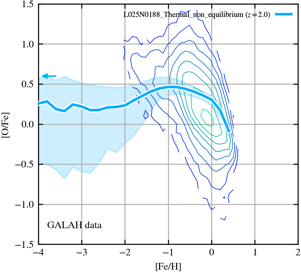
[Fe/H] vs [O/Fe]
[Fe/H] vs [O/Fe] using Asplund et al. (2009) values for [Fe/H]Sun = 7.5 and [O/H]Sun = 8.69. The median [O/Fe] vs median [Fe/H] is indicated by the solid curve(s). The scatter points show abundances of individual stellar particles. The observational data for MW compiles the data from the GALAH survey (Buder et al. 2021). Contours use a log scale with 0.04 bin size and a minimum star count of 10. All recommended flags are applied to GALAH data to select stars (SN, FE/H and X/Fe quality flags). The arrows at [Fe/H]=-4 indicate the median value of [O/Fe] of gas with [Fe/H]<-4.
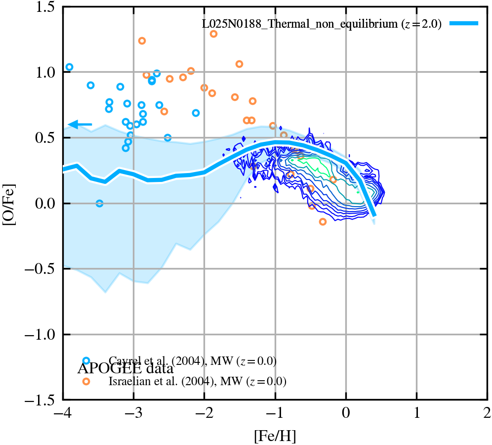
[Fe/H] vs [O/Fe]
[Fe/H] vs [O/Fe] using Asplund et al. (2009) values for [Fe/H]Sun = 7.5 and [O/H]Sun = 8.69. The median [O/Fe] vs median [Fe/H] is indicated by the solid curve(s). The scatter points show abundances of individual stellar particles. The observational data for MW compiles the data from the APOGEE survey (Holtzman et al. 2018) and AstroNN added-value catalog (Leung, H.W. & Bovy, Jo 2019b). We create 6 stellar distributions by selecting stars from APOGEE based on galactocentric radial & azimuthal cuts, and combine them in order to derive a joint stellar abundance distribution that gives less weight to stars in the solar vicinity. The resulting contours use a log scale with 0.2 bin size. The arrows at [Fe/H]=-4 indicate the median value of [O/Fe] of gas with [Fe/H]<-4.
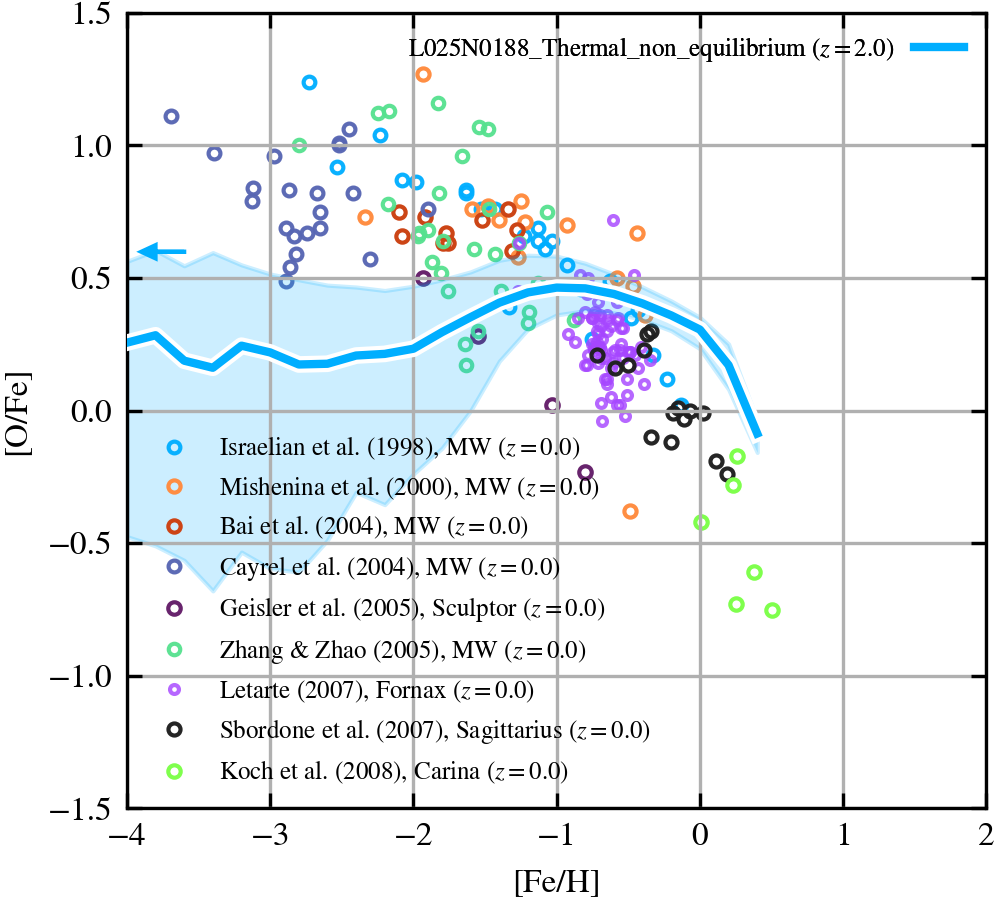
[Fe/H] vs [O/Fe]
[Fe/H] vs [O/Fe] using Asplund et al. (2009) values for [Fe/H]Sun = 7.5 and [O/H]Sun = 8.69. The median [O/Fe] vs median [Fe/H] is indicated by the solid curve(s). The scatter points show abundances of individual stellar particles. The observational data for MW compiles the works of Mishenina+99, Israelian+98, Cayrel+04, Bai+04, Zhang+05, Koch+08. Most of these works assume Grevesser & Anders (1989) values for solar metallicity, their were corrected to Asplund+09. Additional data includes Fornax (Letarte+07), Carina (Kock+05), Sculptor (Geisler+05) and Sagittarious (Sbordone+07). The arrows at [Fe/H]=-4 indicate the median value of [O/Fe] of gas with [Fe/H]<-4.
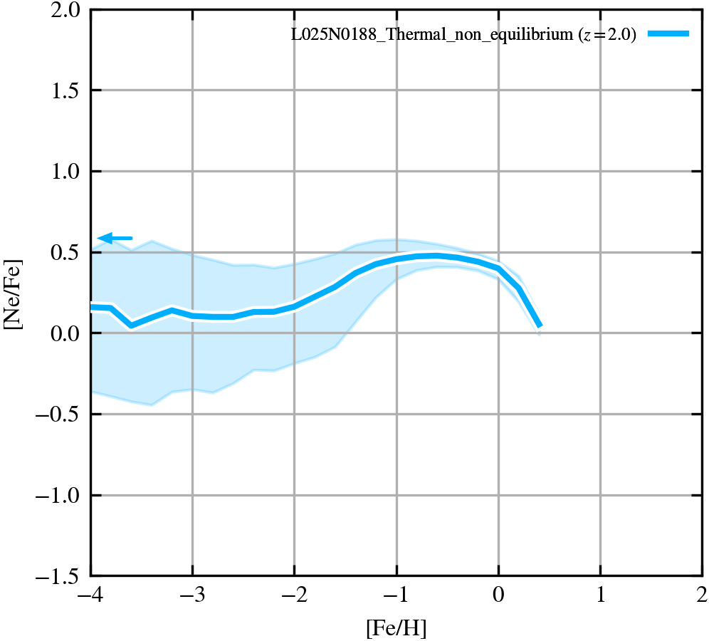
[Fe/H] vs [Ne/Fe]
[Fe/H] vs [Ne/Fe] using Asplund et al. (2009) values for [Fe/H]Sun = 7.5 and [Ne/H]Sun = 7.93. The median [Ne/Fe] vs median [Fe/H] is indicated by the solid curve(s). The scatter points show abundances of individual stellar particles. The arrows at [Fe/H]=-4 indicate the median value of [Ne/Fe] of gas with [Fe/H]<-4.
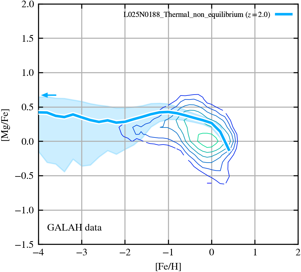
[Fe/H] vs [Mg/Fe]
[Fe/H] vs [Mg/Fe] using Asplund et al. (2009) values for [Fe/H]Sun = 7.5 and [Mg/H]Sun = 7.6. The median [Mg/Fe] vs median [Fe/H] is indicated by the solid curve(s). The scatter points show abundances of individual stellar particles. The observational data for MW compiles the data from the GALAH survey (Buder et al. 2021). Contours use a log scale with 0.04 bin size and a minimum star count of 10. All recommended flags are applied to GALAH data to select stars (SN, FE/H and X/Fe quality flags). The arrows at [Fe/H]=-4 indicate the median value of [Mg/Fe] of gas with [Fe/H]<-4.
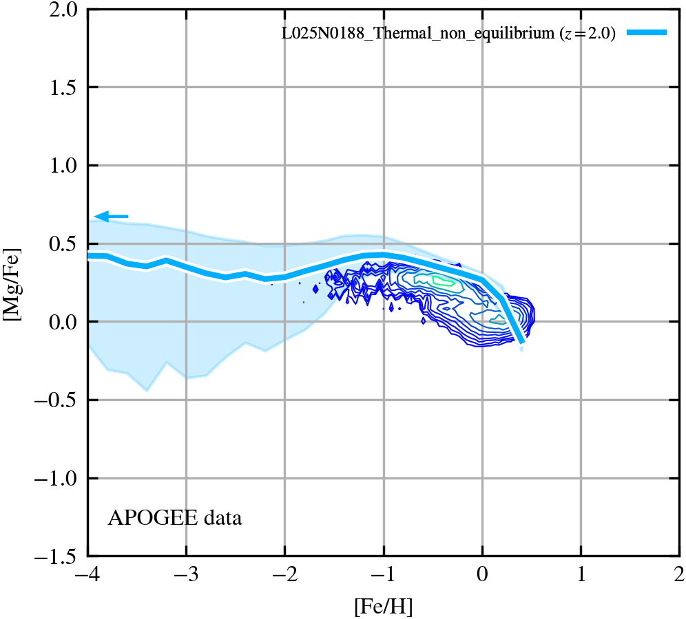
[Fe/H] vs [Mg/Fe]
[Fe/H] vs [Mg/Fe] using Asplund et al. (2009) values for [Fe/H]Sun = 7.5 and [Mg/H]Sun = 7.6. The median [Mg/Fe] vs median [Fe/H] is indicated by the solid curve(s). The scatter points show abundances of individual stellar particles. The observational data for MW compiles the data from the APOGEE survey (Holtzman et al. 2018) and AstroNN added-value catalog (Leung, H.W. & Bovy, Jo 2019b). We create 6 stellar distributions by selecting stars from APOGEE based on galactocentric radial & azimuthal cuts, and combine them in order to derive a joint stellar abundance distribution that gives less weight to stars in the solar vicinity. The resulting contours use a log scale with 0.2 bin size. The arrows at [Fe/H]=-4 indicate the median value of [Mg/Fe] of gas with [Fe/H]<-4.
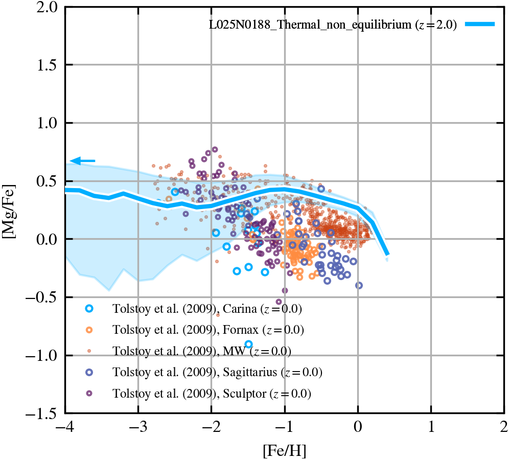
[Fe/H] vs [Mg/Fe]
[Fe/H] vs [Mg/Fe] using Asplund et al. (2009) values for [Fe/H]Sun = 7.5 and [Mg/H]Sun = 7.6. The median [Mg/Fe] vs median [Fe/H] is indicated by the solid curve(s). The scatter points show abundances of individual stellar particles. The observational data for MW, Carina, Fornax, Sculptor and Sagittarious corresponds to a data compilation presented by Tolstoy, Hill & Tosi (2009) and extracted by Rob Crain. Note solar metallicity of Grevesser & Anders (1989) was corrected to Asplund+09. The arrows at [Fe/H]=-4 indicate the median value of [Mg/Fe] of gas with [Fe/H]<-4.
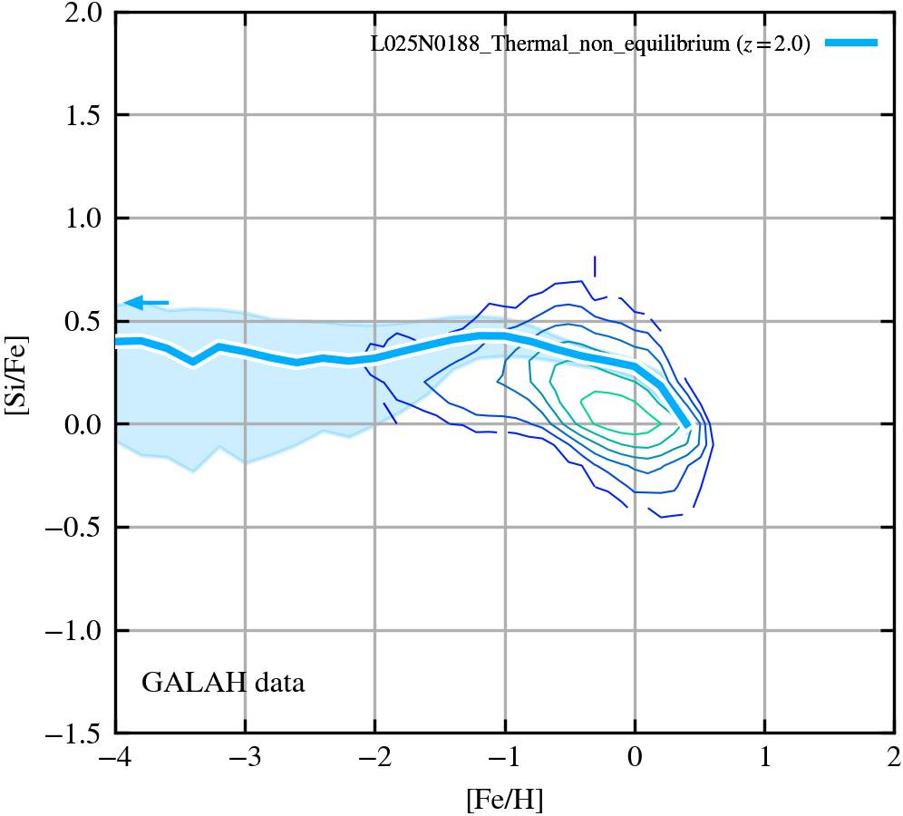
[Fe/H] vs [Si/Fe]
[Fe/H] vs [Si/Fe] using Asplund et al. (2009) values for [Fe/H]Sun = 7.5 and [Si/H]Sun = 7.51. The median [Si/Fe] vs median [Fe/H] is indicated by the solid curve(s). The scatter points show abundances of individual stellar particles. The observational data for MW compiles the data from the GALAH survey (Buder et al. 2021). Contours use a log scale with 0.04 bin size and a minimum star count of 10. All recommended flags are applied to GALAH data to select stars (SN, FE/H and X/Fe quality flags). The arrows at [Fe/H]=-4 indicate the median value of [Si/Fe] of gas with [Fe/H]<-4.
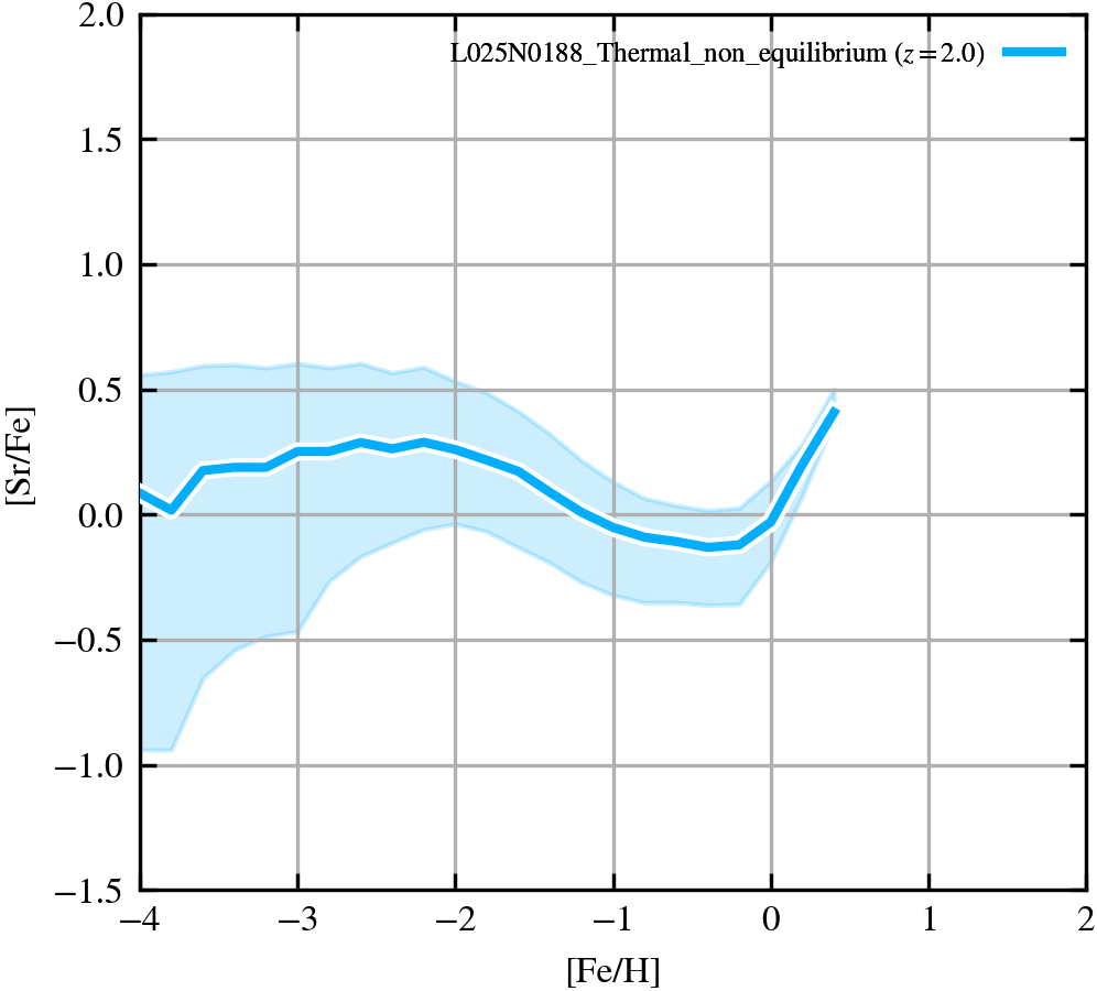
[Fe/H] vs [Sr/Fe]
[Fe/H] vs [Sr/Fe] using Asplund et al. (2009) values for [Fe/H]Sun = 7.5 and [Sr/H]Sun = 2.87. The median [Sr/Fe] vs median [Fe/H] is indicated by the solid curve(s). The scatter points show abundances of individual stellar particles. The arrows at [Fe/H]=-4 indicate the median value of [Sr/Fe] of gas with [Fe/H]<-4.
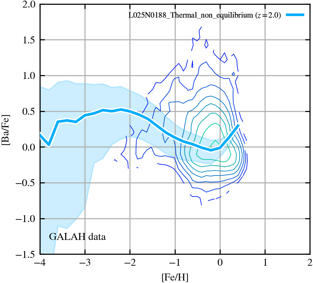
[Fe/H] vs [Ba/Fe]
[Fe/H] vs [Ba/Fe] using Asplund et al. (2009) values for [Fe/H]Sun = 7.5 and [Ba/H]Sun = 2.18. The median [Ba/Fe] vs median [Fe/H] is indicated by the solid curve(s). The scatter points show abundances of individual stellar particles. The observational data for MW compiles the data from the GALAH survey (Buder et al. 2021). Contours use a log scale with 0.04 bin size and a minimum star count of 10. All recommended flags are applied to GALAH data to select stars (SN, FE/H and X/Fe quality flags). The arrows at [Fe/H]=-4 indicate the median value of [Ba/Fe] of gas with [Fe/H]<-4.
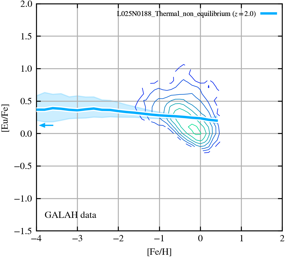
[Fe/H] vs [Eu/Fe]
[Fe/H] vs [Eu/Fe] using Asplund et al. (2009) values for [Fe/H]Sun = 7.5 and [Eu/H]Sun = 0.52. The median [Eu/Fe] vs median [Fe/H] is indicated by the solid curve(s). The scatter points show abundances of individual stellar particles. The observational data for MW compiles the data from the GALAH survey (Buder et al. 2021). Contours use a log scale with 0.04 bin size and a minimum star count of 10. All recommended flags are applied to GALAH data to select stars (SN, FE/H and X/Fe quality flags). The arrows at [Fe/H]=-4 indicate the median value of [Eu/Fe] of gas with [Fe/H]<-4.
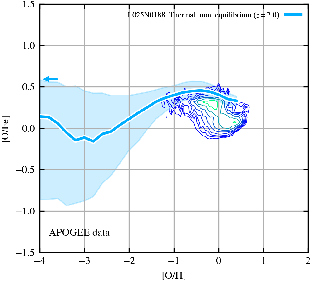
[O/H] vs [O/Fe]
[O/H] vs [O/Fe] using Asplund et al. (2009) values for [Fe/H]Sun = 7.5 and [O/H]Sun = 8.69. The median [O/Fe] vs median [O/H] is indicated by the solid curve(s). The scatter points show abundances of individual stellar particles. The observational data for MW compiles the data from the APOGEE survey (Holtzman et al. 2018) and AstroNN added-value catalog (Leung, H.W. & Bovy, Jo 2019b). We create 6 stellar distributions by selecting stars from APOGEE based on galactocentric radial & azimuthal cuts, and combine them in order to derive a joint stellar abundance distribution that gives less weight to stars in the solar vicinity. The resulting contours use a log scale with 0.2 bin size. The arrows at [O/H]=-4 indicate the median value of [O/Fe] of gas with [O/H]<-4.
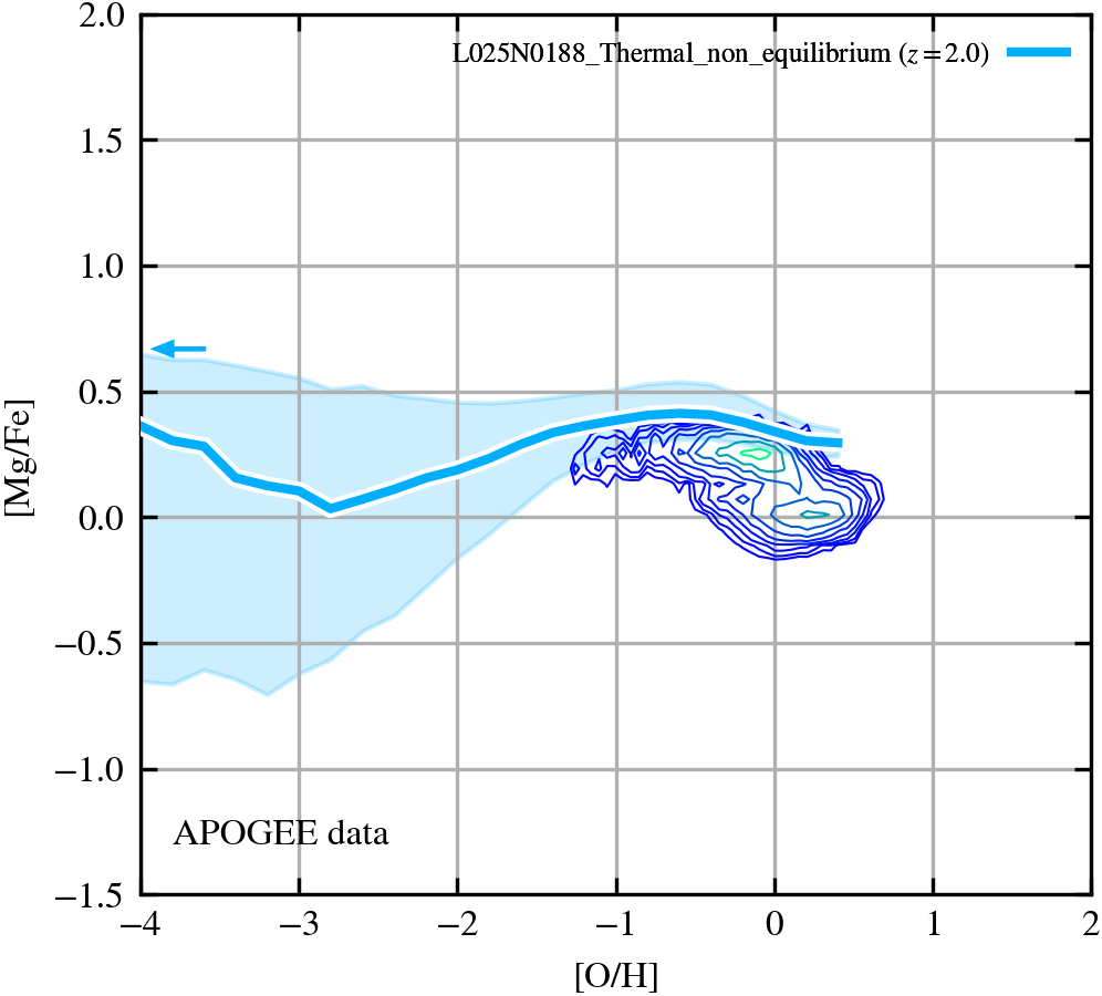
[O/H] vs [Mg/Fe]
[O/H] vs [Mg/Fe] using Asplund et al. (2009) values for [O/H]Sun = 8.69 and [Mg/H]Sun = 7.6. The median [Mg/Fe] vs median [O/H] is indicated by the solid curve(s). The scatter points show abundances of individual stellar particles. The observational data for MW compiles the data from the APOGEE survey (Holtzman et al. 2018) and AstroNN added-value catalog (Leung, H.W. & Bovy, Jo 2019b). We create 6 stellar distributions by selecting stars from APOGEE based on galactocentric radial & azimuthal cuts, and combine them in order to derive a joint stellar abundance distribution that gives less weight to stars in the solar vicinity. The resulting contours use a log scale with 0.2 bin size. The arrows at [O/H]=-4 indicate the median value of [Mg/Fe] of gas with [O/H]<-4.
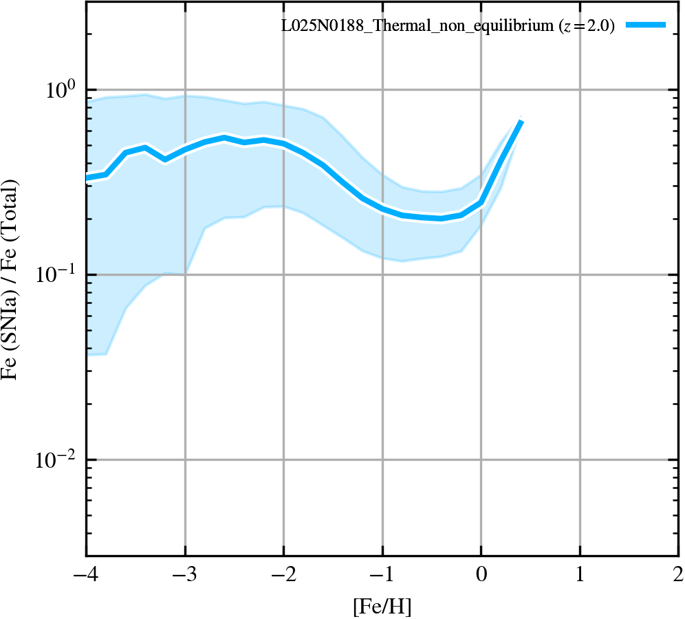
Fraction of Fe from SNIa vs [Fe/H]
The mass fraction of Fe from SNIa vs [Fe/H] using Asplund et al. (2009) values for [Fe/H]Sun = 7.5. The median SNIa Fe fraction vs median [Fe/H] is indicated by the solid curve(s). The scatter points show abundances of individual stellar particles.
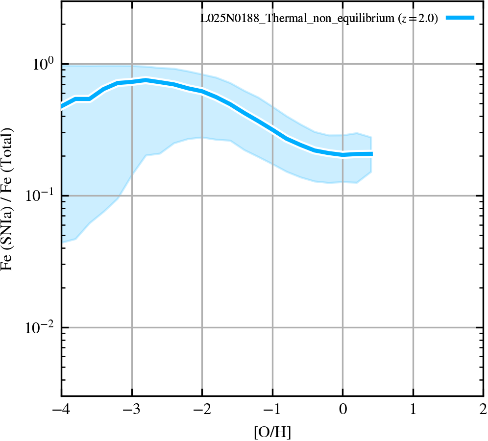
Fraction of Fe from SNIa vs [O/H]
The mass fraction of Fe from SNIa vs [O/H] using Asplund et al. (2009) values for [O/H]Sun = 8.69. The median SNIa Fe fraction vs median [O/H] is indicated by the solid curve(s). The scatter points show abundances of individual stellar particles.
Stellar Metallicity
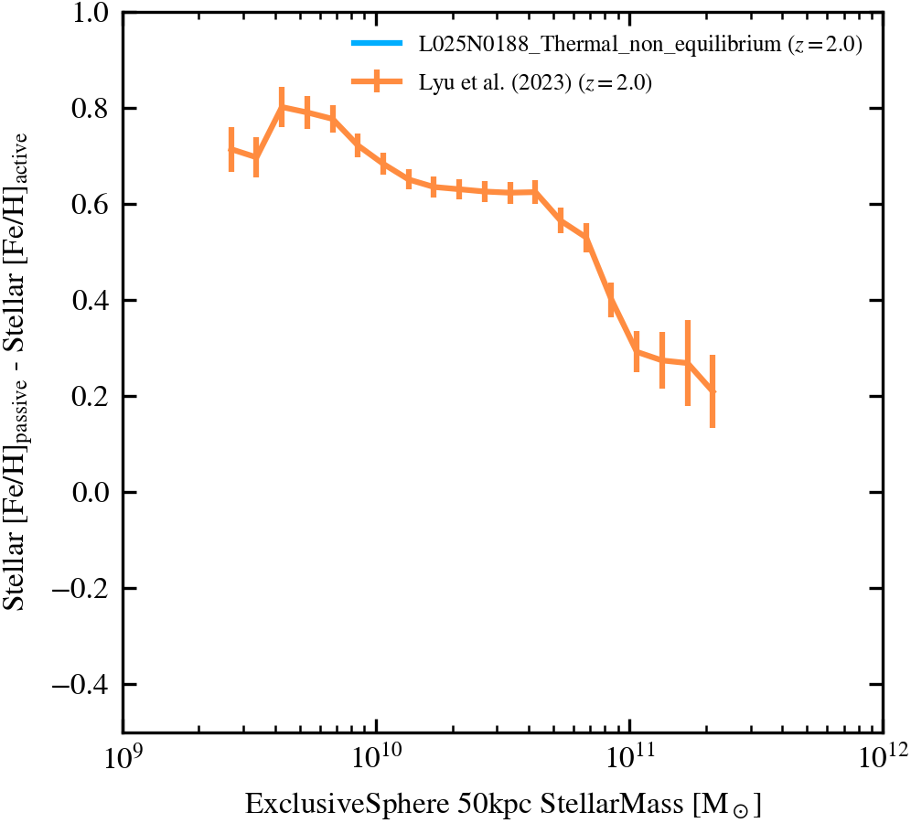
Stellar Metallicity Difference Passive vs. Active Galaxies
The stellar metallicity difference between passive and active central galaxies. The passive (active) metallicity is given by the median metallicity of all galaxies in the mass bin which satisfy the definition of passive (active) galaxies from Lyu+23.
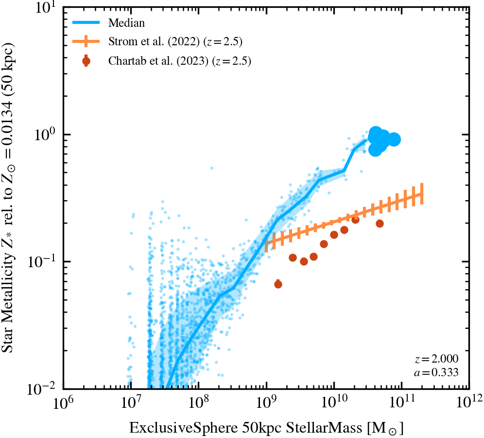
Stellar mass - Star metallicity relation (50 kpc aperture)
Average stellar metallicity measured in the same aperture as the stellar mass. Gallazzi data is corrected from their choice of solar metallicity (0.02) to ours (0.0134). The Yates+ data from MaNGA corresponds to mass-weighted stellar metallicity within 3 arcsec for star-forming galaxies at $z=0$.
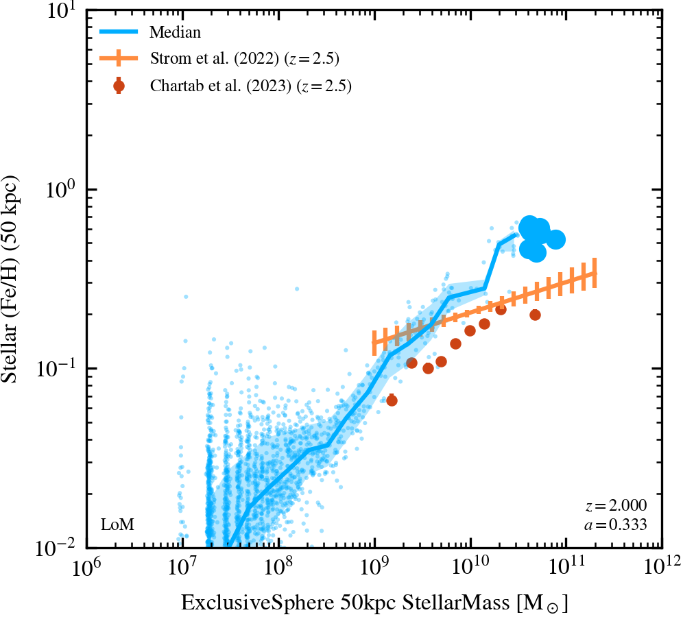
Stellar mass - (Fe/H)$_*$ relation (50 kpc aperture)
Computed as the mass-weighted average of (Fe/H)$_*$, and normalised by solar values. All haloes are plotted, including subhaloes.
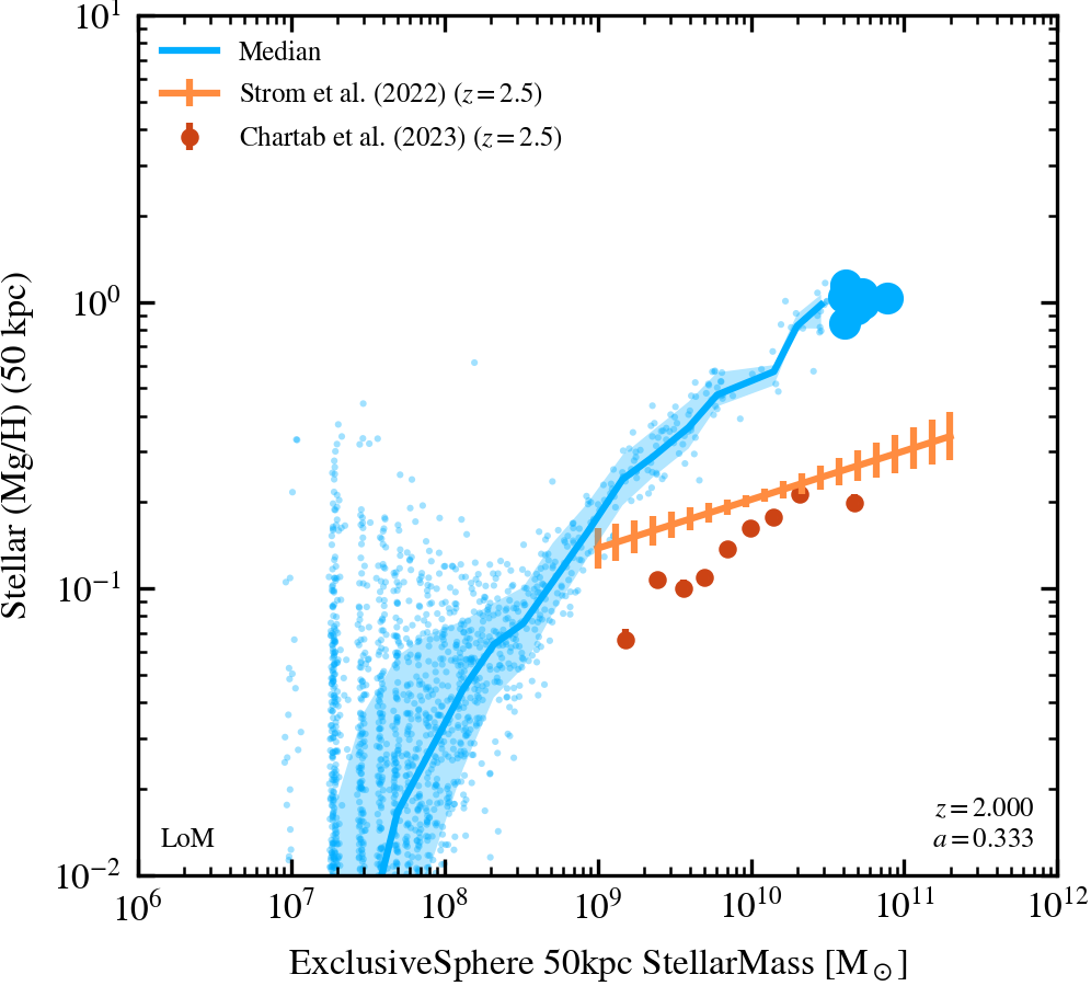
Stellar mass - (Mg/H)$_*$ relation (50 kpc aperture)
Computed as the mass-weighted average of (Mg/H)$_*$, and normalised by solar values. All haloes are plotted, including subhaloes.
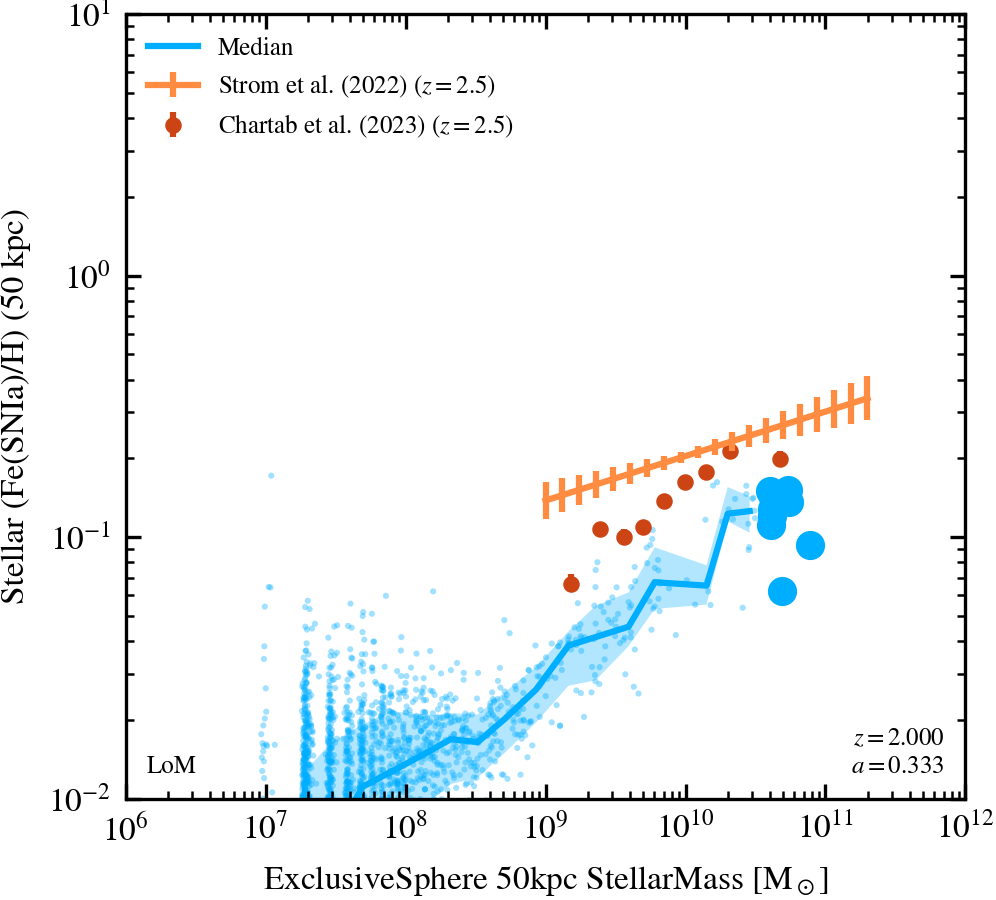
Stellar mass - (Fe$_{\rm SNIa}$/H)$_*$ relation (50 kpc aperture)
Computed as the mass-weighted average of (Fe/H)$_*$, and normalised by solar values. Note that only Fe from SNIa is included. All haloes are plotted, including subhaloes.
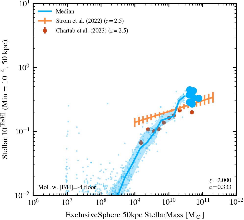
Stellar mass - [Fe/H]$_*$ relation (mean-of-log, 50 kpc aperture)
Computed as the mass-weighted average of log(Fe/H)$_*$, with a floor value set to [Fe/H]=-4. All haloes are plotted, including subhaloes.
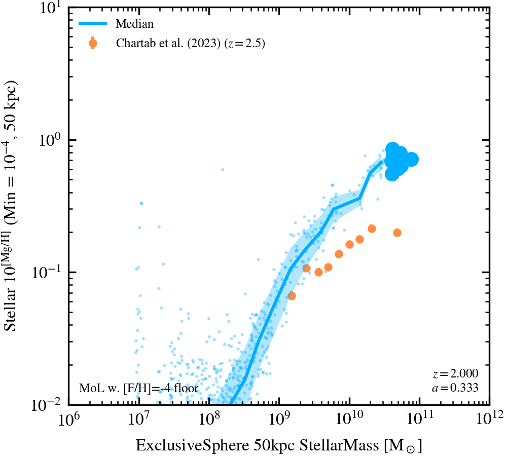
Stellar mass - [Mg/H]$_*$ relation (mean-of-log, 50 kpc aperture)
Computed as the mass-weighted average of log(Mg/H)$_*$, with a floor value set to [Mg/H]=-4. All haloes are plotted, including subhaloes.
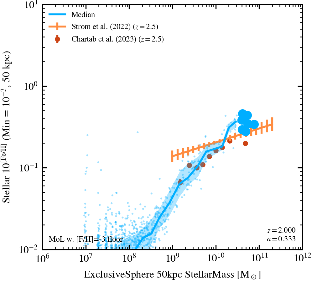
Stellar mass - [Fe/H]$_*$ relation (mean-of-log, 50 kpc aperture)
Computed as the mass-weighted average of log(Fe/H)$_*$, with a floor value set to [Fe/H]=-3. All haloes are plotted, including subhaloes.
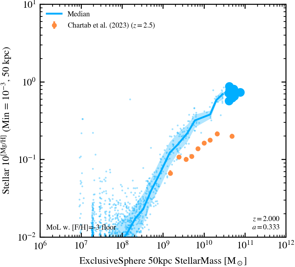
Stellar mass - [Mg/H]$_*$ relation (mean-of-log, 50 kpc aperture)
Computed as the mass-weighted average of log(Mg/H)$_*$, with a floor value set to [Mg/H]=-3. All haloes are plotted, including subhaloes.
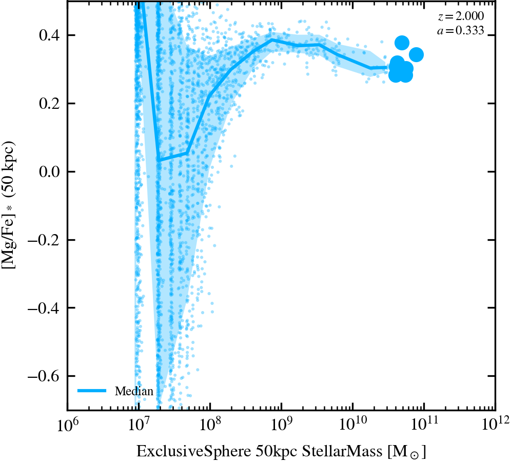
Stellar mass - [Mg/Fe]$_*$ relation (50 kpc aperture)
[Mg/Fe] versus stellar mass, both computed in 50-kpc apertures. The values of [Mg/Fe] are obtained by computing the (log10 of) ratio between the total Magnesium mass in stars and total Iron mass in stars, and then normalising it by the corresponding solar abundances. The solar abundances are taken from Asplund et al. (2009). All haloes are plotted, including subhaloes. Romero-Gomez+ dataset of ATLAS-3D galaxies has been corrected from Grevesse & Sauval (1998) to Aspund+ solar abundances. However Romero-Gomez dataset of dwarf galaxies, that corresponds to a compilation of [alpha/Fe] values from the dwarf spherical galaxies in the Local Group (Table B2 of Romero-Gomez et al. 2023), has not been corrected to Asplund+ solar abundances, this is pending and should be done for each individual data point. Gallazzi+ dataset should be corrected from Grevesse + (1991) to Asplund+ solar abundances. However a different [Fe/H] value is adopted (7.48 as opposed to 7.67) because we think that that value was used in the study, but confirmation from Gallazzi et al. is still pending on this.
Tully-Fisher
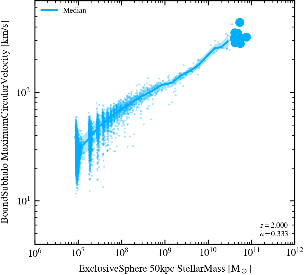
Tully-Fisher (stellar mass, 50 kpc)
The Tully-Fisher relation based on stellar mass.
Stellar mass - Stellar age relation (50 kpc aperture)
Median age of stars within the 50 kpc 3D aperture of each galaxy.
Stellar mass - Stellar age relation (50 kpc aperture, centrals only)
Median age of stars within the 50 kpc 3D aperture of each galaxy, showing central galaxies only.
Stellar mass - Stellar age relation (50 kpc aperture, satellites only)
Median age of stars within the 50 kpc 3D aperture of each galaxy, showing satellite galaxies only.
Halo baryon fractions within $R_{500}$
Baryon (gas + stars) fractions within $R_{500}$ normalised by the cosmic mean. These are 'true' values, i.e. no cut or observational correction was applied.
Halo gas fractions within $R_{500}$ (no hydrostatic bias)
Gas fractions within $R_{500}$ normalised by the cosmic mean. These are 'true' values, i.e. no cut or observational correction was applied. The observational data does not include any correction for hydrostatic bias.
Halo hot gas fractions within $R_{500}$ (no hydrostatic bias)
Fraction of halo mass within $R_{500}$ in hot ($T>10^5$K) gas, normalised by the cosmic mean. These are 'true' values, i.e. no cut or observational correction was applied. The observational data does not include any correction for hydrostatic bias.
Halo gas fractions within $R_{500}$ (with hydrostatic bias)
Gas fractions within $R_{500}$ normalised by the cosmic mean. These are 'true' values, i.e. no cut or observational correction was applied. The observational data was compiled from 10+ HSE data sets (Kugel et al., in prep.), and includes the -0.75 dex hydrostatic bias correction factor used for FLAMINGO.
Halo stellar fractions within $R_{500}$
Stellar fractions within $R_{500}$ normalised by the cosmic mean. These are 'true' values, i.e. no cut or observational correction was applied.
Halo gas masses within $R_{500}$
Gas masses within $R_{500}$. These are 'true' values, i.e. no cut or observational correction was applied.
Black Hole Dynanmical and Subgrid Masses
Relation between black hole particle (dynamical) masses and subgrid masses. The vertical dashed lines shows the primordial gas particle mass and the horizontal dashed lines corresponds to the black hole seed mass.
Cumulative number of AGN thermal injections
The cumulative number of black holes (summed from right to left) with a given total number of thermal energy injections (less than or equal to the number of particles heated) the black hole has had throughout the simulation.
Stellar Mass-Black Hole Mass relation (50 kpc Stellar Mass)
SMBHM relation. Note that the stellar velocity dispersion is measured in observations in a fixed 1 kpc aperture
Stellar Mass-Black Hole Mass relation (50 kpc Stellar Mass)
SMBHM relation. The binned observational data are obtained by combining BH mass measurements for galaxies of different morphologies (Graham 2023) and passive vs. active galaxies (Terrazas et al. 2017) with dependencies on stellar mass of morphological types (Moffett et al. 2016, from the GAMA survey) and quenched fractions (Gilbank et al. 2010, SDSS).
Stellar Mass-Black Hole Mass relation (50 kpc Stellar Mass) for passive central galaxies.
Stellar Mass-Black Hole Mass relation using a 30 kpc stellar mass aperture. Only passive (z=0 sSFR threshold is 0.01 / Gyr, z>0 is 0.2/t_H(z)) central galaxies are included.
Stellar Mass-Black Hole Mass relation (50 kpc Stellar Mass) for active central galaxies.
Stellar Mass-Black Hole Mass relation using a 50 kpc stellar mass aperture. Only active (z=0 sSFR threshold is 0.01 / Gyr, z>0 is 0.2/t_H(z)) central galaxies are included.
Halo Mass-Black Hole Mass relation
Presented for comparison between schemes as halo mass varies significantly less between models and runs.
LOS Stellar Velocity Dispersion-Black Hole Mass relation (10 kpc)
The 3D stellar velocity dispersion is converted into a LOS velocity dispersion using a $1/\sqrt{3}$ correction factor. The stellar velocity dispersion from Sahu et al. (2016) was measured using a fixed 1 kpc aperture, while that from Saglia et al. (2016) was measured using the half-light radius aperture.
Stellar Mass-LOS Stellar Velocity Dispersion relation (10 kpc)
The 3D stellar velocity dispersion is converted into a LOS velocity dispersion using a $1/\sqrt{3}$ correction factor.
Black Hole Mass - sSFR relation (50 kpc sSFR)
Black Hole Mass - sSFR mass relation for galaxies with stellar mass $>10^{10}$ solar masses.
Black Hole Mass Function (adaptive)
The mass function of black holes (active and non-active), using adaptive binning.
Black Hole Eddington Fraction - Mass Relation
The relation between black hole Eddington fraction and subgrid mass.
Black Hole Merger Mass Fractions - Mass Relation
The fraction of subgrid mass growth through mergers versus subgrid mass.
Black Hole Luminosity - Mass Relation
The (instantaneous and bolometric) AGN luminosity versus subgrid mass. Note that this does not include the coupling efficiency factor, i.e. this is not the thermal heating rate.
Black Hole Thermal Energy - Mass Relation
The total AGN injected thermal energies (over the BH lifetime) versus subgrid mass.
Black Hole AGN Bolometric Luminosity Function
The AGN bolometric luminosity function calculated from the accretion rates and radiative efficiencies. The observational data is inferred from different bands using correction factors.
Black Hole AGN Heating Events - Mass Relation
The total number of particles heated by AGN thermal feedback (over the BH lifetime) versus subgrid mass.
sSFR-H$_2$ Fraction
Galaxy H$_2$ mass (including Helium following the observations) over stellar mass as a function of specific star formation rate in 0.2 dex bins, measured in 50 kpc apertures. To include Helium we multiply $M_{\rm H_2}/M_{\rm star}$ by $(1+M_{\rm He}/M_{\rm H})$. The median values are shown.
Stellar Mass Surface Density-H$_2$ Fraction
Galaxy H$_2$ mass (including Helium following the observations) over stellar mass as a function of stellar mass surfaced density in 0.2 dex bins, measured in 50 kpc apertures. To include Helium we multiply $M_{\rm H_2}/M_{\rm star}$ by $(1+M_{\rm He}/M_{\rm H})$. The median values are shown.
sSFR-HI Fraction
Galaxy HI mass over stellar mass as a function of specific star formation rate in 0.2 dex bins, measured in 50 kpc apertures. XGASS (Catinella+18) galaxies are selected to have a flat $M_\star$ distribution in the range $10^9 \; {\rm M_\odot} > M_\star > 10^{10} \; {\rm M_\odot}$, and a higher normalised uniform in the range $10^{10} \; {\rm M_\odot} > M_\star > 10^{11} \; {\rm M_\odot}$.
Stellar Mass Surface Density-HI Fraction
Galaxy HI mass over stellar mass as a function of stellar mass surface density in 0.2 dex bins, measured in 50 kpc apertures. XGASS (Catinella+18) galaxies are selected to have a flat $M_\star$ distribution in the range $10^9 \; {\rm M_\odot} > M_\star > 10^{10} \; {\rm M_\odot}$, and a higher normalised uniform in the range $10^{10} \; {\rm M_\odot} > M_\star > 10^{11} \; {\rm M_\odot}$.
Stellar Mass-H$_2$ Fraction
Galaxy H$_2$ mass (including Helium following the observations) over stellar mass as a function of stellar mass in 0.2 dex bins, measured in 50 kpc apertures. To include Helium we multiply $M_{\rm H_2}/M_{\rm star}$ by $(1+M_{\rm He}/M_{\rm H})$. The median values are shown. In Saintonge2017+ data, all galaxies with $10^9 < M_{\rm star} / \mathrm{M_\odot} < 10^{10}$ have $M_{\rm H_2}/M_{\rm star}$ fractions that cannot be lower than $0.025$, and for galaxies with $M_{\rm star} / \mathrm{M_\odot} > 10^{10}$ the floor value is $0.015$. The median values ("Binning") are shown.
Stellar Mass-HI Fraction
Galaxy HI mass over stellar mass as a function of stellar mass in 0.2 dex bins, measured in 50 kpc apertures. LITTLE THINGS galaxies are dIrrs selected to be within 10 Mpc, with 50$\%$ of galaxies within 3.6 Mpc, and detected in HI. MAGMA (Hunt+20) are selected on both CO and HI detecions, but find the galaxies down to $10^7 \; {\rm M_\odot}$ consistent with the extrapolated SFMS (i.e. typical star-forming galaxies). XGASS (Catinella+18) galaxies are selected to have a flat $M_\star$ distribution in the range $10^9 \; {\rm M_\odot} > M_\star > 10^{10} \; {\rm M_\odot}$, and a higher normalised uniform in the range $10^{10} \; {\rm M_\odot} > M_\star > 10^{11} \; {\rm M_\odot}$.
Stellar Mass-HI Fraction (active galaxies)
Galaxy HI mass over stellar mass as a function of stellar mass in 0.2 dex bins, measured in 50 kpc apertures. Active galaxies only.
sSFR-Cold gas Fraction
Galaxy neutral gas mass over stellar mass as a function of specific star formation rate, with adaptive binning, measured in 50 kpc apertures. XGASS (Catinella+18) galaxies are selected to have a flat $M_\star$ distribution in the range $10^9 \; {\rm M_\odot} > M_\star > 10^{10} \; {\rm M_\odot}$, and a higher normalised uniform in the range $10^{10} \; {\rm M_\odot} > M_\star > 10^{11} \; {\rm M_\odot}$.
Stellar Mass-Cold gas Fraction
Galaxy H$_2$ mass over neutral gas (HI+H$_2$) mass as a function of stellar mass in 0.2 dex bins, measured in 50 kpc apertures. MAGMA (Hunt+20) are selected on both CO and HI detecions, but find the galaxies down to $10^7 \; {\rm M_\odot}$ consistent with the extrapolated SFMS (i.e. typical star-forming galaxies). XGASS and XCOLDGASS samples are uniform in mass in the range $10^9 \; {\rm M_\odot} > M_\star > 10^{10} \; {\rm M_\odot}$ and $10^{10} \; {\rm M_\odot} > M_\star > 10^{11} \; {\rm M_\odot}$ and plotting those above the CO detection limit ($M_{\rm H2}/M_*$ > $1.5\%$).
sSFR-Neutral Fraction
Galaxy H$_2$ mass over neutral gas mass (HI+H$_2$) as a function of specific star formation rate, with adaptive binning, measured in 50 kpc apertures. XCOLDGASS (Saintonge+17) and XGASS (Catinella+18) galaxies are selected to have a flat $M_\star$ distribution in the range $10^9 \; {\rm M_\odot} > M_\star > 10^{10} \; {\rm M_\odot}$, and a higher normalised uniform in the range $10^{10} \; {\rm M_\odot} > M_\star > 10^{11} \; {\rm M_\odot}$.
Atomic Gas Mass Evolution
Evolution of the atomic gas mass abundance plotted directly from the statistics.txt file produced by SWIFT, compared with assorted observational estimates corrected to our cosmology. The simulation data is corrected for Helium by multiplying it by 1/0.76.
Molecular Gas Mass Evolution
Evolution of the molecular gas mass abundance plotted directly from the statistics.txt file produced by SWIFT, compared with assorted observational estimates.
sSFR-Neutral Gas to SF Gas Fraction (50 kpc aperture)
Only active galaxies are included in the median line. Fraction is HI + H$_2$ mass over stellar mass in a 50 kpc aperture.
sSFR-HI Gas to SF Gas Fraction (50 kpc aperture)
Only active galaxies are included in the median line. Fraction is HI mass over stellar mass in a 50 kpc aperture.
sSFR-H$_2$ Gas to SF Gas Fraction (50 kpc aperture)
Only active galaxies are included in the median line. Fraction is H$_2$ mass over stellar mass in a 50 kpc aperture.
Stellar Mass-Neutral Gas to Baryonic Fraction (50 kpc aperture)
All galaxies are included in the median line. Fraction is HI + H$_2$ mass over total baryonic mass in a 50 kpc aperture.
Stellar Mass-HI to Neutral Gas Fraction (50 kpc aperture)
Only active galaxies are included in the median line. Fraction is HI mass over HI + H$_2$ mass in a 50 kpc aperture.
Stellar Mass-H$_2$ to Neutral Gas Fraction (50 kpc aperture)
Only active galaxies are included in the median line. Fraction is H$_2$ mass over HI + H$_2$ mass in a 50 kpc aperture.
Stellar Mass-H$_2$ to SF Gas Fraction (50 kpc aperture)
Only active galaxies are included in the median line. Fraction is H$_2$ gas mass over SF gas in a 50 kpc aperture.
Stellar Mass-HI Gas Mass Relation (50 kpc aperture)
All galaxies are included in the median line. Both stellar and HI masses were computed in 50 kpc apertures.
Stellar Mass-HI Gas Mass Relation (50 kpc aperture)
Only active galaxies are included in the median line. Both stellar and HI masses were computed in 50 kpc apertures.
Stellar Mass-H$_2$ Gas Mass Relation (50 kpc aperture)
All galaxies are included in the median line. H$_2$ mass was corrected for Helium. Both stellar and H$_2$ masses were computed in 50 kpc apertures.
Stellar Mass-H$_2$ Gas Mass Relation (50 kpc aperture)
Only active galaxies are included in the median line. H$_2$ mass was corrected for Helium. Both stellar and H$_2$ masses were computed in 50 kpc apertures.
Halo Mass-HI Gas Mass Relation (50 kpc aperture)
All galaxies are included in the median line. HI mass was computed in 50 kpc apertures.
Halo Mass-H$_2$ Gas Mass Relation (50 kpc aperture)
All galaxies are included in the median line. H$_2$ mass was corrected for Helium. H$_2$ mass was computed in 50 kpc apertures.
HI Column Density Distribution Function (full box, full range)
The column density distribution function of neutral hydrogen computed by projecting the entire box along the z-axis, corrected for the size of the box in redshift space.
HI Column Density Distribution Function (half box, full range)
The column density distribution function of neutral hydrogen computed by splitting the box in half along the z-axis and projecting each half separately, also along the z-axis. Corrected for the size of the box in redshift space.
HI Column Density Distribution Function (full box, reduced range)
The column density distribution function of neutral hydrogen computed by projecting the entire box along the z-axis, corrected for the size of the box in redshift space.
HI Column Density Distribution Function (half box, reduced range)
The column density distribution function of neutral hydrogen computed by splitting the box in half along the z-axis and projecting each half separately, also along the z-axis. Corrected for the size of the box in redshift space.
HeII Column Density Distribution Function (full box, full range)
The column density distribution function of singly-ionized helium computed by projecting the entire box along the z-axis, corrected for the size of the box in redshift space.
HeII Column Density Distribution Function (half box, full range)
The column density distribution function of singly-ionized helium computed by splitting the box in half along the z-axis and projecting each half separately, also along the z-axis. Corrected for the size of the box in redshift space.
HeII Column Density Distribution Function (full box, reduced range)
The column density distribution function of singly-ionized helium computed by projecting the entire box along the z-axis, corrected for the size of the box in redshift space.
HeII Column Density Distribution Function (half box, reduced range)
The column density distribution function of singly-ionized helium computed by splitting the box in half along the z-axis and projecting each half separately, also along the z-axis. Corrected for the size of the box in redshift space.
Density-Temperature
Density-temperature diagram. If present, dashed line represents the entropy floor (equation of state).
Density-Temperature (Star Forming Gas)
Density-temperature diagram shaded by the mass fraction of the gas whose instantaneous star formation rate is greater than zero.
Density-Temperature (Metals)
Density-temperature diagram with the pixel value weighted by the mean logarithmic metal mass fraction (absolute) in that bin. Medians are not used due to their computational complexity. If present, dashed line represents the entropy floor (equation of state).
Density-Temperature (Dust)
Density-temperature diagram with the pixel value weighted by the mean logarithmic dust mass fraction in that bin. Medians are not used due to their computational complexity.
Density-Temperature (Dust / Metals)
Density-temperature diagram with the pixel value the ratio of dust to metals for the particles within that bin (i.e. the values are binned weighted by dust, then by metals, and those two grids are divided to produce the dust to metals ratio). Only particles with a metal mass fraction of $Z > 10^{-8}$ are plotted.
Dust-to-metal Ratio
Density-temperature diagram shaded by the total fraction of metals in the dust phase.
Density-Internal Energy
Density-Internal Energy diagram. If present, dashed line represents the entropy floor (equation of state).
Density-Pressure
Density-pressure diagram. If present, dashed line represents the entropy floor (equation of state).
Density-Median Temperature
Median temperature as a function of density for all gas and for gas in selected metallicity ranges.
Oxygen abundance vs dust-to-gas ratio in Neutral Gas (30 kpc aperture)
Dust-to-gas mass ratio as a function of oxygen number density abundance in Neutral gas. Only active galaxies are selected.
Oxygen abundance vs dust-to-gas ratio in Neutral Gas (30 kpc aperture)
Dust-to-gas mass ratio as a function of oxygen number density abundance in Neutral gas. Only galaxies that are active and have $M_* > 10^9 \, \rm M_\odot$ are selected.
Oxygen abundance (from Z) vs dust-to-gas ratio in Neutral Gas (30 kpc aperture)
Dust-to-gas mass ratio as a function of metallicity represented as an oxygen number density abundance for compatibility with observations. Only active galaxies are selected.
Oxygen abundance vs dust-to-metal ratio in Neutral Gas (30 kpc aperture)
Dust-to-metal mass ratio as a function of oxygen number density abundance in Neutral gas. Only active galaxies are selected.
Oxygen abundance vs dust-to-metal ratio in Neutral Gas (30 kpc aperture)
Dust-to-metal mass ratio as a function of oxygen number density abundance in Neutral gas. Only galaxies that are active and have $M_* > 10^9 \, \rm M_\odot$ are selected.
Oxygen abundance (from Z) vs dust-to-metal ratio in Neutral Gas (30 kpc aperture)
Dust-to-metal mass ratio as a function of metallicity, converted into an oxygen number density abundance for compatability with observations. Only active galaxies are selected.
Dust Mass Density Evolution
Evolution of the dust mass density plotted directly from the statistics.txt file produced by SWIFT.
Stellar mass vs Small-to-Large Ratio
The dust mass ratio of small to large grains in all gas aggregated over a 50kpc radius aperture in galaxies. Compared to values derived from observation by Relano et al 2020.
Stellar mass vs Small-to-Large Ratio (H2 only)
The dust mass ratio of small to large grains in all gas aggregated over a 50kpc radius aperture in galaxies. Compared to values derived from observation by Relano et al 2020.
Stellar mass vs Dust Mass
Gas-phase dust mass as a function of stellar mass, high redshift data individual galaxies from ALESS ALMA SMG survey (Da Cunha et al 2015). Data redshifts are photometric.
Star formation rate vs Dust Mass
Gas-phase dust mass as a function of SFR, comparing to local Dustpedia galaxies with properties derived using the CIGALE SED fitting code (Bianchi et al 2018)
Neutral Gas Mass vs Dust Mass
Gas-phase dust mass as a function of SFR, comparing to local Dustpedia galaxies with properties derived using the CIGALE SED fitting code (Bianchi et al 2018)
Molecular Gas Mass vs Dust Mass
Gas-phase dust mass as a function of SFR, comparing to local Dustpedia galaxies with properties derived using the CIGALE SED fitting code (Bianchi et al 2018)
Dust Mass Function
50 kpc aperture Galaxy Dust Mass Function, showing all galaxies with a fixed bin-width of 0.2 dex.
Dust Mass Function
50 kpc aperture Galaxy Dust Mass Function, showing all galaxies with an adaptive bin-width.
Molecular Dust Mass Function
30 kpc aperture Galaxy Dust Mass Function, showing all galaxies with a fixed bin-width of 0.2 dex.
Neutral Dust Mass Function
30 kpc aperture Galaxy Dust Mass Function, showing all galaxies with a fixed bin-width of 0.2 dex.
Cold Dense Dust Mass Function
30 kpc aperture Galaxy Dust Mass Function, showing all galaxies with a fixed bin-width of 0.2 dex.
HI-to-stellar mass ratio vs dust-to-stellar mass ratio in neutral gas.
HI to stellar mass ratio as a function of the dust-to-stellar mass ratio in neutral gas measured in 50kpc apertures, and applying a JINGLE-like mass selection.
HI-to-stellar mass ratio vs dust-to-metal ratio in cold, dense gas
HI to stellar mass ratio as a function of the dust-to-metal ratio in cold, dense gas ($T < 10^{4.5}\;{\rm K}$, $n_{\rm H} > 0.1 \; {\rm cm^{-3}}$) measured in 50kpc apertures, and applying a JINGLE-like mass selection.
HI-to-stellar mass ratio vs Oxygen abundance
HI to stellar mass ratio as a function of the gas-phase Oxygen abundance measured in 50 kpc apertures, and applying a JINGLE-like mass selection.
Density of the gas heated by SNII
Distributions of the gas densities recorded when the gas was last heated by SNII, split by redshift. The y axis shows the number of SNII-heated gas particles per bin divided by the bin width and by the total of SNII-heated gas particles. The dashed vertical lines show the median SNII gas-densities, while the dotted lines indicade the critical density from C. Dalla Vecchia & J. Schaye (2012) for SN min and max heating temperatures with $f_t=10$. Star particles are not included.
Density of the gas heated by AGN
Distributions of the gas densities recorded when the gas was last heated by AGN, split by redshift. The y axis shows the number of AGN-heated gas particles per bin divided by the bin width and by the total of AGN-heated gas particles. The dashed vertical lines show the median AGN gas-densities, while the dotted lines indicade the critical density from C. Dalla Vecchia & J. Schaye (2012) for AGN heating temperature with $f_t=10$. Star particles not included.
Maximal SNII thermal feedback Density-Stellar Mass relation
Includes all haloes, including subhaloes.
Maximal SNII thermal feedback Density-Maximal Stellar Birth Density relation
Includes all haloes, including subhaloes.
Kick velocity distribution at last SNII
Distributions of SNII kick velocities experienced by the gas recorded when the gas was last kicked by SNII, split by redshift. The y axis shows the number of SNII-kicked gas particles per bin divided by the bin width and by the total of SNII-kicked gas particles. The dashed vertical lines show the median kick velocitites, while the dotted lines indicade the target kick velocity. Star particles are not included.
Maximal SNII kick velocity
Maximal SNII kick velocities by experienced by particles in SNII kinetic feedback throughout the entire simulation.
H$_2$ Mass Function
H$_2$ MF, showing all galaxies with a fixed bin-width of 0.2 dex. H$_2$ mass corrected for Helium (uses H$_2$ masses in 50 kpc apertures)
H$_2$ Mass Function
H$_2$ MF, showing all galaxies with an adaptive bin-width. H$_2$ mass corrected for Helium (uses H$_2$ masses in 50 kpc apertures)
Stellar mass - Gas diffuse metallicity relation (log-of-mean, from Z, 50 kpc aperture)
Only shown for star forming galaxies. Computed as the average mass-weighted metal mass fraction (converted to 12 + $\log_{10}$ O/H by assuming solar abundance patterns) of cold, dense gas ($T < 10^{4.5}\;{\rm K}$, $n_{\rm H} > 0.1 \; {\rm cm^{-3}}$). No minimum metallicity is imposed. All haloes are plotted, including subhaloes. This uses depleted gas metallicity, i.e. it does not include metals that are present in dust.
Stellar mass - Gas diffuse metallicity relation (log-of-mean, 50 kpc aperture)
Only shown for star forming galaxies. Represented by 12 + $\log_{10}$ O/H (where O/H is linearly averaged for diffuse O) of the cold, dense gas ($T < 10^{4.5}\;{\rm K}$, $n_{\rm H} > 0.1 \; {\rm cm^{-3}}$). No minimum metallicity is imposed. All haloes are plotted, including subhaloes. This uses depleted gas metallicity, i.e. it does not include metals that are present in dust.
Stellar mass - Gas (Diffuse + Dust) metallicity relation (log-of-mean, 50 kpc aperture)
Only shown for star forming galaxies. Represented by 12 + $\log_{10}$ O/H (where O/H is linearly averaged for total O) of the cold, dense gas ($T < 10^{4.5}\;{\rm K}$, $n_{\rm H} > 0.1 \; {\rm cm^{-3}}$). No minimum metallicity is imposed. All haloes are plotted, including subhaloes. This uses undepleted gas metallicity, i.e. it includes metals that are present in dust.
Stellar mass - Gas diffuse metallicity relation (mean-of-log, 50 kpc aperture)
Only shown for star forming galaxies. Represented by 12 + $\log_{10}$ O/H (where $\log_{10}$ O/H is averaged between gas particles with a [O/H]=-4 floor and diffuse O) of the cold, dense gas ($T < 10^{4.5}\;{\rm K}$, $n_{\rm H} > 0.1 \; {\rm cm^{-3}}$). All haloes are plotted, including subhaloes. This uses depleted gas metallicity, i.e. it does not include metals that are present in dust.
Stellar mass - Gas diffuse metallicity relation (mean-of-log, 50 kpc aperture)
Only shown for star forming galaxies. Represented by 12 + $\log_{10}$ O/H (where $\log_{10}$ O/H is averaged between gas particles with a [O/H]=-3 floor for diffuse O) of the cold, dense gas ($T < 10^{4.5}\;{\rm K}$, $n_{\rm H} > 0.1 \; {\rm cm^{-3}}$). All haloes are plotted, including subhaloes. This uses depleted gas metallicity, i.e. it does not include metals that are present in dust.
Stellar mass - Gas diffuse metallicity relation (log-of-mean, 50 kpc aperture)
Only shown for galaxies with cold, dense gas. Represented by 12 + $\log_{10}$ O/H (where O/H is linearly averaged for diffuse O) of the cold, dense gas ($T < 10^{4.5}\;{\rm K}$, $n_{\rm H} > 0.1 \; {\rm cm^{-3}}$). No minimum metallicity is imposed. All haloes are plotted, including subhaloes. This uses depleted gas metallicity, i.e. it does not include metals that are present in dust.
Halo Mass Function ($M_{200, crit}$)
Halo masses are masses within the over-density radius enclosing 200x the critical density, using 0.2 dex fixed bin-widths (centrals only).
Halo Mass Function ($M_{200, crit}$)
Halo masses are masses within the over-density radius enclosing 200x the critical density, using adaptive binning (centrals only).
Gas Particle Masses
Gas Particle Masses with the threshold for splitting indicated by the vertical dashed line.
Gas Particle Smoothing Lengths
Gas Particle Comoving Smoothing Lengths with the minimal smoothing length indicated by the vertical dashed line.
Gas Particle Minimal Smoothing Lengths
Gas Particle Comoving Minimal Smoothing Lengths reached during the simulation, split by redshifts at which these minimal smoothing lengths were reached and normalised by the gravitational softening length (at the corresponding redshift). The minimal allowed ratio between smoothing length and gravitational softening length is indicated by the vertical dashed line. The normalisation by the softening includes the factor of 3 to convert from the Plummer-equivalent softening length, which is specified in the parameter file. The normalisation also accounts for the factor of $\gamma_{\rm kernel} \approx 2$, which relates the smoothing length to the extent of an SPH kernel.
Gas Particle Minimal Smoothing Lengths vs. Redshift
Gas Particle Comoving Minimal Smoothing Lengths versus Redshifts at which these minimal smoothing lengths were reached. The black dashed and black dotted curves indicate, respectively, the minimum allowed smoothing length and gravitational softening length at a given redshift.
Stellar Mass Histogram (50 kpc aperture)
Cumulative histogram of stellar masses using the same bins as the mass function.
Star Formation Rate Histogram (50 kpc aperture)
Cumulative histogram of star formation rates using the same bins as the star formation rates function.
H$_2$
Density-temperature diagram shaded by H$_2$ mass fraction. The fraction is computed as the H$_2$ mass contained in each cell over the mass of gas in that cell.
HI
Density-temperature diagram shaded by HI mass fraction. The fraction is computed as the HI mass contained in each cell over the mass of gas in that cell.
HII
Density-temperature diagram shaded by HII mass fraction. The fraction is computed as the HII mass contained in each cell over the mass of gas in that cell.
Hydrogen Phase Fractions
Co-plot of species fractions (left y-axis) and the dust-to-metal ratio (right y-axis) as a function opf gas density. If available, solid green line shows explicitly modelled dust-to-metal ratio, while dashed green is interpolated from the Ploeckinger+20 tables.
Hydrogen Phase Fractions (Depletion Fraction)
Co-plot of species fractions (left y-axis) and the dust-to-metal ratio (right y-axis) as a function of gas density. If available, solid green line shows explicitly modelled dust-to-metal ratio, while dashed green is interpolated from the Ploeckinger+20 tables.
Hydrogen Phase Fractions (Diffuse Fraction)
Co-plot of species fractions (left y-axis) and the dust-to-metal ratio (right y-axis) as a function of gas density. If available, solid green line shows explicitly modelled dust-to-metal ratio, while dashed green is interpolated from the Ploeckinger+20 tables.
u-band Luminosity Function (50 kpc aperture)
50 kpc aperture dust-free rest-frame luminosity function in the GAMA u-band, constructed using the Trayford et al. (2015) model, showing all galaxies with a fixed bin-width of 0.2 dex.
g-band Luminosity Function (50 kpc aperture)
50 kpc aperture dust-free rest-frame luminosity function in the GAMA g-band, constructed using the Trayford et al. (2015) model, showing all galaxies with a fixed bin-width of 0.2 dex.
r-band Luminosity Function (50 kpc aperture)
50 kpc aperture dust-free rest-frame luminosity function in the GAMA r-band, constructed using the Trayford et al. (2015) model, showing all galaxies with a fixed bin-width of 0.2 dex.
i-band Luminosity Function (50 kpc aperture)
50 kpc aperture dust-free rest-frame luminosity function in the GAMA i-band, constructed using the Trayford et al. (2015) model, showing all galaxies with a fixed bin-width of 0.2 dex.
z-band Luminosity Function (50 kpc aperture)
50 kpc aperture dust-free rest-frame luminosity function in the GAMA z-band, constructed using the Trayford et al. (2015) model, showing all galaxies with a fixed bin-width of 0.2 dex.
Y-band Luminosity Function (50 kpc aperture)
50 kpc aperture dust-free rest-frame luminosity function in the GAMA Y-band, constructed using the Trayford et al. (2015) model, showing all galaxies with a fixed bin-width of 0.2 dex.
J-band Luminosity Function (50 kpc aperture)
50 kpc aperture dust-free rest-frame luminosity function in the GAMA J-band, constructed using the Trayford et al. (2015) model, showing all galaxies with a fixed bin-width of 0.2 dex.
H-band Luminosity Function (50 kpc aperture)
50 kpc aperture dust-free rest-frame luminosity function in the GAMA H-band, constructed using the Trayford et al. (2015) model, showing all galaxies with a fixed bin-width of 0.2 dex.
K-band Luminosity Function (50 kpc aperture)
50 kpc aperture dust-free rest-frame luminosity function in the GAMA K-band, constructed using the Trayford et al. (2015) model, showing all galaxies with a fixed bin-width of 0.2 dex.
Maximal Temperature reached by gas particles
Maximal temperature recorded by gas particles throughout the entire simulation.
Maximal Temperature-Redshift
The maximal temperatures reached by all star and gas particles (density given by the colour map) against the redshift at which they were at that temperature.
Gas Phase Metal Mass Density Evolution
Evolution of the metal mass in gas per unit co-moving volume.
Metal Mass Locked in Stars Density Evolution
Evolution of the metal mass locked in stars per unit co-moving volume.
Metal Mass Locked in Black Holes Density Evolution
Evolution of the metal mass locked in black holes per unit co-moving volume.
Metal Mass Fraction Distribution
Metal mass fraction distribution shown for each simulation; solid lines show gas metallicity and dashed lines show the same for the stars. If present, dashed line represents the entropy floor (equation of state). The percentages in between brackets indicate what fraction of the particles is above the lower limit and hence included in the distribution.
Wall-clock time per gas particle updates.
Wall-clock time to run a time-step as a function of the number of gas particles updated. The tracks at the top correspond to steps where the tree is rebuilt, i/o is performed, FoF is run or other non-regular operations are done.
The number of steps vs. wall-clock time
The cumulative number of the simulation time-steps as a function of the wall-clock time.
Number of steps vs. cosmic time
The cumulative number of the simulation time-steps as a function of the cosmic time.
Wall-clock time per time-bin
Total wall-clock time spent in each of the different simulation time-bins.
Dead time fraction vs scale factor
Evolution of the dead time fraction as a function of scale factor. The dashed line represents the average dead time over the entire run.
Satellite Fraction
The fraction of galaxies which are satellites as a function of their stellar mass
Satellite Fraction (Passive galaxies)
The fraction of passive galaxies which are satellites as a function of their stellar mass
Stellar Mass-(Projected) Galaxy Size relation (50 kpc aperture)
Uses stellar sizes calculated from a projected distribution within a 50 kpc aperture.
Stellar Mass-(Projected) Galaxy Size relation (50 kpc aperture, calibration)
Uses stellar sizes calculated from a projected distribution within a 50 kpc aperture. The comparison data is used for calibration.
Stellar Mass-(Projected) Galaxy Size relation (50 kpc aperture)
Only shows active galaxies defined based on their sSFRs. Both Lange et al. (2015) and van der Wel et al. (2014) use the semi-major half-light radius of the best-fitting Sérsic model as the definition of galaxy size, while Mosleh et al. (2020) use the circularized half-light radius.
Stellar Mass-(Projected) Galaxy Size relation (50 kpc aperture)
Only shows passive galaxies defined based on their sSFRs. Both Lange et al. (2015) and van der Wel et al. (2014) use the semi-major half-light radius of the best-fitting Sérsic model as the definition of galaxy size, while Mosleh et al. (2020) use the circularized half-light radius.
SNII Energy Fraction Distribution
Distribution of SNII energy fractions, split by redshift. The y-axis shows the number of stars per bin divided by the bin width and by the total number of stars. The dashed vertical lines show the median SNII energy fraction in three different redshift intervals. The dotted vertical line shows the average SNII energy fraction computed over all star particles in the simulation.
SNII Energy Fraction vs. Stellar Birth Pressure
The relation between the SNII energy fraction and stellar birth pressure. The dashed vertical lines indicate the pivot birth pressure used in the simulation.
SNII Energy Fraction vs. Galaxy Stellar Mass
The SNII energy fraction evaluated at the galaxy median stellar birth pressure vs. galaxy stellar mass. The solid lines indicate the median values in stellar mass bins, while the shaded regions indicate the 16-84 percentile scatter.
Stellar Mass-SNIa rate relation (active only, 50 kpc aperture)
Uses a 50 kpc 3D aperture and only active galaxies.
Stellar Mass-SNIa rate relation (passive only, 50 kpc aperture)
Uses a 50 kpc 3D aperture and only passive galaxies.
Stellar Mass-SNIa rate per stellar mass relation (active only, 50 kpc aperture)
Uses a 50 kpc 3D aperture.
Stellar Mass-SNIa rate per stellar mass relation (passive only, 50 kpc aperture)
Uses a 50 kpc 3D aperture.
Gas metallicity-SNIa rate per stellar mass relation (active only, 50 kpc aperture)
Uses a 50 kpc 3D aperture, active galaxies only with a stellar mass above 1e10 Msun.
Gas metallicity-SNIa rate per stellar mass relation (active only, 50 kpc aperture)
Uses a 50 kpc 3D aperture, active galaxies only with a stellar mass above 5e10 Msun.
SFR-SNIa rate per stellar mass relation (50 kpc aperture)
Uses a 50 kpc 3D aperture, only select galaxies with a stellar mass above 1e10 Msun.
SFR-SNIa rate per stellar mass relation (50 kpc aperture)
Uses a 50 kpc 3D aperture, only select galaxies with a stellar mass above 5e10 Msun.
sSFR-SNIa rate per stellar mass relation (50 kpc aperture)
Uses a 50 kpc 3D aperture, only select galaxies with a stellar mass above 1e10 Msun.
sSFR-SNIa rate per stellar mass relation (50 kpc aperture)
Uses a 50 kpc 3D aperture, only select galaxies with a stellar mass above 5e10 Msun.
Star Formation History
Star formation density history plotted directly from the SFR.txt file produced by SWIFT.
Stellar Mass Density Evolution
Evolution of the stellar mass density plotted directly from the statistics.txt file produced by SWIFT.
Stellar Mass-Star Formation Rate (50 kpc aperture) for active galaxies.
Only active galaxies are included. SFRs from Koprowski+ are based on UV+IV; active galaxies in Koprowski+ were identified based on UVJ colour selection.
Specific Star Formation Rate - Stellar Mass (50 kpc aperture)
All galaxies, including those deemed to be passive (z=0 sSFR threshold is 0.01 / Gyr, z>0 is 0.2/t_H(z)), are included in the median line.
Specific Star Formation Rate - Stellar Mass (50 kpc aperture, centrals only)
Only central galaxies are included in the median line.
Specific Star Formation Rate - Stellar Mass (50 kpc aperture, satellites only)
Only satellite galaxies are included in the median line.
Specific Star Formation Rate - Stellar Mass (50 kpc aperture, active only)
Only active galaxies (z=0 sSFR threshold is 0.01 / Gyr, z>0 is 0.2/t_H(z)) are included in the median line.
Passive Fraction - Stellar Mass (50 kpc aperture)
The sSFR threshold to determine if a galaxy is passsive is 0.01 / Gyr for z=0, 0.2/t_H(z) for z>0.
Passive Fraction - Stellar Mass (50 kpc aperture, with scatter)
The sSFR threshold to determine if a galaxy is passsive is 0.01 / Gyr for z=0, 0.2/t_H(z) for z>0. All stellar masses contain an additional 0.3 dex log-normal scatter.
Passive Fraction - Stellar Mass (50 kpc aperture, centrals)
The sSFR threshold to determine if a galaxy is passsive is 0.01 / Gyr for z=0, 0.2/t_H(z) for z>0. This figure shows only central galaxies
Passive Fraction - Stellar Mass (50 kpc aperture, satellites)
The sSFR threshold to determine if a galaxy is passsive is 0.01 / Gyr for z=0, 0.2/t_H(z) for z>0. This figure shows only satellite galaxies
Star Formation Rate Function (50 kpc aperture)
50 kpc aperture galaxy star formation rate function, showing all galaxies with a fixed bin-width of 0.2 dex.
Star Formation Rate Function (50 kpc aperture)
50 kpc aperture galaxy star formation rate function, showing all galaxies with an adaptive bin-width.
Stellar Birth Densities
Distributions of stellar birth densities, split by redshift. The y axis shows the number of stars per bin divided by the bin width and by the total number of stars. The dashed vertical lines show the median stellar birth-densities, while the dotted lines indicade the critical density from C. Dalla Vecchia & J. Schaye (2012) for SN min and max heating temperatures with $f_t=10$.
Stellar Birth Pressures
Distributions of stellar birth pressures, split by redshift. The y axis shows the number of stars per bin divided by the bin width and by the total number of stars. The dashed vertical lines show the median stellar birth-pressures.
Stellar Birth Temperatures
Distributions of stellar birth temperatures, split by redshift. The y axis shows the number of stars per bin divided by the bin width and by the total number of stars. The dashed vertical lines show the median stellar birth-temperatures.
Stellar Birth Velocity Dispersions
Distributions of stellar birth velocity dispersions, split by redshift. The y axis shows the number of stars per bin divided by the bin width and by the total number of stars. The dashed vertical lines show the median stellar birth velocity dispersions.
Stellar Birth Densities-Metallicity
Stellar birth densities vs metallicity diagram. The pixel colour indicates the number of stellar particles in the pixel. At a given birth density, particles with metallicities lower than the smallest value along the Y axis are placed in the lowest-metallicity bin. MMF stands for metal mass fraction.
Stellar Birth Densities-Birth Redshift
Stellar birth densities vs birth redshift diagram. The pixel colour indicates the number of stellar particles in the pixel.
Stellar Metallicity-Birth Redshift
Stellar metallicity vs birth redshift diagram. The pixel colour indicates the number of stellar particles in the pixel. At a given birth redshift, particles with metallicities lower than the smallest value along the X axis are placed in the lowest-metallicity bin.
Stellar Birth Densities-Stellar Birth Temperatures
Stellar birth densities vs Stellar birth temperature diagram. The pixel colour indicates the number of stellar particles in the pixel.
Median Stellar Birth Pressure-Stellar Mass relation
Includes all haloes, including subhaloes. The median is calculated based on the entire set of stellar particles within each (sub)halo.
Median Stellar Birth Density-Stellar Mass relation
Includes all haloes, including subhaloes. The median is calculated based on the entire set of stellar particles within each (sub)halo.
Median Stellar Birth Temperature-Stellar Mass relation
Includes all haloes, including subhaloes. The median is calculated based on the entire set of stellar particles within each (sub)halo.
Stellar Mass Function (50 kpc aperture)
50 kpc aperture GSMF, showing all galaxies with a fixed bin-width of 0.2 dex.
Stellar Mass Function (50 kpc aperture, centrals only)
50 kpc aperture GSMF, showing central galaxies only, with a fixed bin-width of 0.2 dex.
Stellar Mass Function (50 kpc aperture, satellites only)
50 kpc aperture GSMF, showing satellite galaxies only, with a fixed bin-width of 0.2 dex.
Stellar Mass Function (50 kpc aperture)
50 kpc aperture GSMF, showing all galaxies with a fixed bin-width of 0.2 dex. Only Leja et al. (2020) and Driver et al. (2021) data are shown.
Stellar Mass Function (50 kpc aperture, adaptive)
50 kpc aperture GSMF, showing all galaxies with an adaptive bin-width.
Stellar Mass Function (50 kpc aperture, adaptive)
50 kpc aperture GSMF, showing all galaxies with an adaptive bin-width. Only Leja et al. (2020) and Driver et al. (2021) data are shown.
Stellar Mass Function (50 kpc aperture, adaptive, 25->50 Mpc box size correction)
50 kpc aperture GSMF, showing all galaxies with an adaptive bin-width. The data have been corrected to a box size of 50 Mpc, assuming the original simulation used a 25 Mpc box.
Stellar Mass Function (50 kpc aperture, adaptive, 25->50 Mpc box size correction)
50 kpc aperture GSMF, showing all galaxies with an adaptive bin-width. The data have been corrected to a box size of 50 Mpc, assuming the original simulation used a 25 Mpc box. Only Leja et al. (2020) and Driver et al. (2021) data are shown.
Stellar Mass Function (50 kpc aperture, with scatter)
50 kpc aperture GSMF, showing all galaxies with a fixed bin-width of 0.2 dex, with an additional 0.3 dex log-normal scatter in the stellar mass.
Stellar Mass Function (50 kpc aperture, with scatter)
50 kpc aperture GSMF, showing all galaxies with a fixed bin-width of 0.2 dex, with an additional 0.3 dex log-normal scatter in the stellar mass. Only Leja et al. (2020) and Driver et al. (2021) data are shown.
Stellar Mass Function (50 kpc aperture, adaptive, with scatter)
50 kpc aperture GSMF, showing all galaxies with an adaptive bin-width, with an additional 0.3 dex log-normal scatter in the stellar mass.
Stellar Mass Function (50 kpc aperture, adaptive, with scatter)
50 kpc aperture GSMF, showing all galaxies with an adaptive bin-width, with an additional 0.3 dex log-normal scatter in the stellar mass. Only Leja et al. (2020) and Driver et al. (2021) data are shown.
Stellar Mass-Halo Mass relation (ratio, 100 kpc aperture, $M_{200,crit}$, centrals only)
Includes only central haloes.
Stellar Mass-Halo Mass relation (ratio, 100 kpc aperture, $M_{\rm BN98}$, centrals only)
Includes only central haloes.
Stellar Mass-Halo Mass relation (ratio, 50 kpc aperture, $M_{\rm BN98}$, centrals only)
Includes only central haloes.
Stellar Mass-Halo Mass relation (ratio, 30 kpc aperture, $M_{\rm BN98}$, centrals only)
Includes only central haloes.
Stellar Mass-Halo Mass relation (ratio, 100 kpc aperture, $M_{200,crit}$, centrals only, stellar x-axis)
Includes only central haloes.
Stellar Mass-Halo Mass relation (ratio, 100 kpc aperture, $M_{\rm BN98}$, centrals only, stellar x-axis)
Includes only central haloes.
Stellar Mass-Halo Mass relation (ratio, 50 kpc aperture, $M_{\rm BN98}$, centrals only, stellar x-axis)
Includes only central haloes.
Stellar Mass-Halo Mass relation (ratio, 30 kpc aperture, $M_{\rm BN98}$, centrals only, stellar x-axis)
Includes only central haloes.
Stellar Mass-Halo Mass relation (100 kpc aperture, $M_{200,crit}$)
Includes all haloes, including subhaloes.
Stellar Mass-Halo Mass relation (100 kpc aperture, $M_{\rm BN98}$)
Includes all haloes, including subhaloes.
Stellar Mass-Halo Mass relation (10 kpc 2D aperture, $M_{200,crit}$, centrals only)
Includes only central haloes, and excludes the contribution of satellites in projection, for both the simulated and observed data. The halo masses in observations by DeMaio et al. (2020) and the semi-empirical model by Huang et al. (2022) were converted from the $M_{500}$ and $M_\mathrm{BN98}$ definitions, respectively, to a $M_{200}$ definition (critical overdensity), by assuming an NFW profile and concentration $c=5$. The halo masses from Golden-Marx et al. (2022) were converted from a mean overdensity to critical overdensity (factor 200) definition. None of the halo masses are corrected for (hydrostatic and other) bias. The IMF from observations by Golden-Marx et al. (2022) was converted from Salpeter to Chabrier. Cosmology corrections were not needed. The data that are of intermediate-redshift objects can be used for comparison here because the evolution of BCG stellar cores is observed to be negligible in this regime. The Huang et al. (2022) model is tailored to groups and clusters, and uses aperture definitions for stellar masses, not only for its predictions but also for the observational data used for calibration.
Stellar Mass-Halo Mass relation (30 kpc 2D aperture, $M_{200,crit}$, centrals only)
Includes only central haloes, and excludes the contribution of satellites in projection, for both the simulated and observed data. The halo masses in observations by Kravstov et al. (2018) and the semi-empirical model by Huang et al. (2022) were converted from the $M_{500}$ and $M_\mathrm{BN98}$ definitions, respectively, to a $M_{200}$ definition (critical overdensity), by assuming an NFW profile and concentration $c=5$. The halo masses from Golden-Marx et al. (2022) were converted from a mean overdensity to critical overdensity (factor 200) definition. None of the halo masses are corrected for (hydrostatic and other) bias. The IMF from observations by Golden-Marx et al. (2022) was converted from Salpeter to Chabrier. Cosmology corrections were not needed. The data that are of intermediate-redshift objects can be used for comparison here because the evolution of BCG stellar cores is observed to be negligible in this regime. The Huang et al. (2022) model is tailored to groups and clusters, and uses aperture definitions for stellar masses, not only for its predictions but also for the observational data used for calibration.
Stellar Mass-Halo Mass relation (50 kpc 2D aperture, $M_{200,crit}$, centrals only)
Includes only central haloes, and excludes the contribution of satellites in projection, for both the simulated and observed data. The halo masses in observations by Gonzalez et al. (2013) and Kravstov et al. (2018), as well as the semi-empirical model by Huang et al. (2022), were converted from the $M_{500}$ and $M_\mathrm{BN98}$ definitions to a $M_{200}$ definition (critical overdensity), by assuming an NFW profile and concentration $c=5$. The halo masses from Golden-Marx et al. (2022) were converted from a mean overdensity to critical overdensity (factor 200) definition. None of the halo masses are corrected for (hydrostatic and other) bias. The IMF from observations by Golden-Marx et al. (2022) was converted from Salpeter to Chabrier. Cosmology corrections were not needed. The data that are of intermediate-redshift objects can may be a slight underestimate due to weak growth of the ICL with redshift. The Huang et al. (2022) model is tailored to groups and clusters, and uses aperture definitions for stellar masses, not only for its predictions but also for the observational data used for calibration.
Stellar Mass-Halo Mass relation (100 kpc 2D aperture, $M_{200,crit}$, centrals only)
Includes only central haloes, and excludes the contribution of satellites in projection, for both the simulated and observed data. The halo masses in observations by Kravstov et al. (2018) and DeMaio et al. (2020), as well as the semi-empirical model by Huang et al. (2022), were converted from the $M_{500}$ and $M_\mathrm{BN98}$ definitions to a $M_{200}$ definition (using the critical overdensity), by assuming an NFW profile and concentration $c=5$. The halo masses from Golden-Marx et al. (2022) were converted from a mean overdensity to critical overdensity (factor 200) definition. None of the halo masses are corrected for (hydrostatic and other) bias. The IMF from observations by Golden-Marx et al. (2022) was converted from Salpeter to Chabrier. Cosmology corrections were not needed. The data that are of intermediate-redshift objects are likely a slight underestimate due to weak growth of the ICL with redshift. The Huang et al. (2022) model is tailored to groups and clusters, and uses aperture definitions for stellar masses, not only for its predictions but also for the observational data used for calibration.
[Fe/H] vs [C/Fe]
[Fe/H] vs [C/Fe] using Asplund et al. (2009) values for [Fe/H]Sun = 7.5 and [C/H]Sun = 8.43. The median [C/Fe] vs median [Fe/H] is indicated by the solid curve(s). The scatter points show abundances of individual stellar particles. The observational data for MW compiles the data from the GALAH survey (Buder et al. 2021). Contours use a log scale with 0.04 bin size and a minimum star count of 10. All recommended flags are applied to GALAH data to select stars (SN, FE/H and X/Fe quality flags). The arrows at [Fe/H]=-4 indicate the median value of [C/Fe] of gas with [Fe/H]<-4.
[Fe/H] vs [C/Fe]
[Fe/H] vs [C/Fe] using Asplund et al. (2009) values for [Fe/H]Sun = 7.5 and [C/H]Sun = 8.43. The median [C/Fe] vs median [Fe/H] is indicated by the solid curve(s). The scatter points show abundances of individual stellar particles. The observational data for MW compiles the data from the APOGEE survey (Holtzman et al. 2018) and AstroNN added-value catalog (Leung, H.W. & Bovy, Jo 2019b). We create 6 stellar distributions by selecting stars from APOGEE based on galactocentric radial & azimuthal cuts, and combine them in order to derive a joint stellar abundance distribution that gives less weight to stars in the solar vicinity. The resulting contours use a log scale with 0.2 bin size. The arrows at [Fe/H]=-4 indicate the median value of [C/Fe] of gas with [Fe/H]<-4.
[Fe/H] vs [C/O]
[Fe/H] vs [C/O] using Asplund et al. (2009) values for [O/H]Sun = 8.69 and [C/H]Sun = 8.43. The median [C/O] vs median [Fe/H] is indicated by the solid curve(s). The scatter points show abundances of individual stellar particles. The observational data for MW compiles the data from the APOGEE survey (Holtzman et al. 2018) and AstroNN added-value catalog (Leung, H.W. & Bovy, Jo 2019b). We create 6 stellar distributions by selecting stars from APOGEE based on galactocentric radial & azimuthal cuts, and combine them in order to derive a joint stellar abundance distribution that gives less weight to stars in the solar vicinity. The resulting contours use a log scale with 0.2 bin size. The arrows at [Fe/H]=-4 indicate the median value of [C/O] of gas with [Fe/H]<-4.
[O/H] vs [C/O]
[O/H] vs [C/O] using Asplund et al. (2009) values for [O/H]Sun = 8.69 and [C/H]Sun = 8.43. The median [C/O] vs median [O/H] is indicated by the solid curve(s). The scatter points show abundances of individual stellar particles. The observational data for MW compiles the data from the APOGEE survey (Holtzman et al. 2018) and AstroNN added-value catalog (Leung, H.W. & Bovy, Jo 2019b). We create 6 stellar distributions by selecting stars from APOGEE based on galactocentric radial & azimuthal cuts, and combine them in order to derive a joint stellar abundance distribution that gives less weight to stars in the solar vicinity. The resulting contours use a log scale with 0.2 bin size. The arrows at [O/H]=-4 indicate the median value of [C/O] of gas with [O/H]<-4.
[Fe/H] vs [N/Fe]
[Fe/H] vs [N/Fe] using Asplund et al. (2009) values for [Fe/H]Sun = 7.5 and [N/H]Sun = 7.83. The median [N/Fe] vs median [Fe/H] is indicated by the solid curve(s). The scatter points show abundances of individual stellar particles. The observational data for MW compiles the data from the APOGEE survey (Holtzman et al. 2018) and AstroNN added-value catalog (Leung, H.W. & Bovy, Jo 2019b). We create 6 stellar distributions by selecting stars from APOGEE based on galactocentric radial & azimuthal cuts, and combine them in order to derive a joint stellar abundance distribution that gives less weight to stars in the solar vicinity. The resulting contours use a log scale with 0.2 bin size. The arrows at [Fe/H]=-4 indicate the median value of [N/Fe] of gas with [Fe/H]<-4.
[O/H] vs [N/O]
[O/H] vs [N/O] using Asplund et al. (2009) values for [O/H]Sun = 8.69 and [N/H]Sun = 7.83. The median [N/O] vs median [O/H] is indicated by the solid curve(s). The scatter points show abundances of individual stellar particles. The observational data for MW compiles the data from the APOGEE survey (Holtzman et al. 2018) and AstroNN added-value catalog (Leung, H.W. & Bovy, Jo 2019b). We create 6 stellar distributions by selecting stars from APOGEE based on galactocentric radial & azimuthal cuts, and combine them in order to derive a joint stellar abundance distribution that gives less weight to stars in the solar vicinity. The resulting contours use a log scale with 0.2 bin size. The arrows at [O/H]=-4 indicate the median value of [N/O] of gas with [O/H]<-4.
[Fe/H] vs [N/O]
[Fe/H] vs [N/O] using Asplund et al. (2009) values for [Fe/H]Sun = 7.5, [N/H]Sun = 7.83 and [O/H]Sun = 8.69. The median [N/O] vs median [Fe/H] is indicated by the solid curve(s). The scatter points show abundances of individual stellar particles. The observational data for MW compiles the data from the APOGEE survey (Holtzman et al. 2018) and AstroNN added-value catalog (Leung, H.W. & Bovy, Jo 2019b). We create 6 stellar distributions by selecting stars from APOGEE based on galactocentric radial & azimuthal cuts, and combine them in order to derive a joint stellar abundance distribution that gives less weight to stars in the solar vicinity. The resulting contours use a log scale with 0.2 bin size. The arrows at [Fe/H]=-4 indicate the median value of [N/O] of gas with [O/H]<-4.
[Fe/H] vs [O/Fe]
[Fe/H] vs [O/Fe] using Asplund et al. (2009) values for [Fe/H]Sun = 7.5 and [O/H]Sun = 8.69. The median [O/Fe] vs median [Fe/H] is indicated by the solid curve(s). The scatter points show abundances of individual stellar particles. The observational data for MW compiles the data from the GALAH survey (Buder et al. 2021). Contours use a log scale with 0.04 bin size and a minimum star count of 10. All recommended flags are applied to GALAH data to select stars (SN, FE/H and X/Fe quality flags). The arrows at [Fe/H]=-4 indicate the median value of [O/Fe] of gas with [Fe/H]<-4.
[Fe/H] vs [O/Fe]
[Fe/H] vs [O/Fe] using Asplund et al. (2009) values for [Fe/H]Sun = 7.5 and [O/H]Sun = 8.69. The median [O/Fe] vs median [Fe/H] is indicated by the solid curve(s). The scatter points show abundances of individual stellar particles. The observational data for MW compiles the data from the APOGEE survey (Holtzman et al. 2018) and AstroNN added-value catalog (Leung, H.W. & Bovy, Jo 2019b). We create 6 stellar distributions by selecting stars from APOGEE based on galactocentric radial & azimuthal cuts, and combine them in order to derive a joint stellar abundance distribution that gives less weight to stars in the solar vicinity. The resulting contours use a log scale with 0.2 bin size. The arrows at [Fe/H]=-4 indicate the median value of [O/Fe] of gas with [Fe/H]<-4.
[Fe/H] vs [O/Fe]
[Fe/H] vs [O/Fe] using Asplund et al. (2009) values for [Fe/H]Sun = 7.5 and [O/H]Sun = 8.69. The median [O/Fe] vs median [Fe/H] is indicated by the solid curve(s). The scatter points show abundances of individual stellar particles. The observational data for MW compiles the works of Mishenina+99, Israelian+98, Cayrel+04, Bai+04, Zhang+05, Koch+08. Most of these works assume Grevesser & Anders (1989) values for solar metallicity, their were corrected to Asplund+09. Additional data includes Fornax (Letarte+07), Carina (Kock+05), Sculptor (Geisler+05) and Sagittarious (Sbordone+07). The arrows at [Fe/H]=-4 indicate the median value of [O/Fe] of gas with [Fe/H]<-4.
[Fe/H] vs [Ne/Fe]
[Fe/H] vs [Ne/Fe] using Asplund et al. (2009) values for [Fe/H]Sun = 7.5 and [Ne/H]Sun = 7.93. The median [Ne/Fe] vs median [Fe/H] is indicated by the solid curve(s). The scatter points show abundances of individual stellar particles. The arrows at [Fe/H]=-4 indicate the median value of [Ne/Fe] of gas with [Fe/H]<-4.
[Fe/H] vs [Mg/Fe]
[Fe/H] vs [Mg/Fe] using Asplund et al. (2009) values for [Fe/H]Sun = 7.5 and [Mg/H]Sun = 7.6. The median [Mg/Fe] vs median [Fe/H] is indicated by the solid curve(s). The scatter points show abundances of individual stellar particles. The observational data for MW compiles the data from the GALAH survey (Buder et al. 2021). Contours use a log scale with 0.04 bin size and a minimum star count of 10. All recommended flags are applied to GALAH data to select stars (SN, FE/H and X/Fe quality flags). The arrows at [Fe/H]=-4 indicate the median value of [Mg/Fe] of gas with [Fe/H]<-4.
[Fe/H] vs [Mg/Fe]
[Fe/H] vs [Mg/Fe] using Asplund et al. (2009) values for [Fe/H]Sun = 7.5 and [Mg/H]Sun = 7.6. The median [Mg/Fe] vs median [Fe/H] is indicated by the solid curve(s). The scatter points show abundances of individual stellar particles. The observational data for MW compiles the data from the APOGEE survey (Holtzman et al. 2018) and AstroNN added-value catalog (Leung, H.W. & Bovy, Jo 2019b). We create 6 stellar distributions by selecting stars from APOGEE based on galactocentric radial & azimuthal cuts, and combine them in order to derive a joint stellar abundance distribution that gives less weight to stars in the solar vicinity. The resulting contours use a log scale with 0.2 bin size. The arrows at [Fe/H]=-4 indicate the median value of [Mg/Fe] of gas with [Fe/H]<-4.
[Fe/H] vs [Mg/Fe]
[Fe/H] vs [Mg/Fe] using Asplund et al. (2009) values for [Fe/H]Sun = 7.5 and [Mg/H]Sun = 7.6. The median [Mg/Fe] vs median [Fe/H] is indicated by the solid curve(s). The scatter points show abundances of individual stellar particles. The observational data for MW, Carina, Fornax, Sculptor and Sagittarious corresponds to a data compilation presented by Tolstoy, Hill & Tosi (2009) and extracted by Rob Crain. Note solar metallicity of Grevesser & Anders (1989) was corrected to Asplund+09. The arrows at [Fe/H]=-4 indicate the median value of [Mg/Fe] of gas with [Fe/H]<-4.
[Fe/H] vs [Si/Fe]
[Fe/H] vs [Si/Fe] using Asplund et al. (2009) values for [Fe/H]Sun = 7.5 and [Si/H]Sun = 7.51. The median [Si/Fe] vs median [Fe/H] is indicated by the solid curve(s). The scatter points show abundances of individual stellar particles. The observational data for MW compiles the data from the GALAH survey (Buder et al. 2021). Contours use a log scale with 0.04 bin size and a minimum star count of 10. All recommended flags are applied to GALAH data to select stars (SN, FE/H and X/Fe quality flags). The arrows at [Fe/H]=-4 indicate the median value of [Si/Fe] of gas with [Fe/H]<-4.
[Fe/H] vs [Sr/Fe]
[Fe/H] vs [Sr/Fe] using Asplund et al. (2009) values for [Fe/H]Sun = 7.5 and [Sr/H]Sun = 2.87. The median [Sr/Fe] vs median [Fe/H] is indicated by the solid curve(s). The scatter points show abundances of individual stellar particles. The arrows at [Fe/H]=-4 indicate the median value of [Sr/Fe] of gas with [Fe/H]<-4.
[Fe/H] vs [Ba/Fe]
[Fe/H] vs [Ba/Fe] using Asplund et al. (2009) values for [Fe/H]Sun = 7.5 and [Ba/H]Sun = 2.18. The median [Ba/Fe] vs median [Fe/H] is indicated by the solid curve(s). The scatter points show abundances of individual stellar particles. The observational data for MW compiles the data from the GALAH survey (Buder et al. 2021). Contours use a log scale with 0.04 bin size and a minimum star count of 10. All recommended flags are applied to GALAH data to select stars (SN, FE/H and X/Fe quality flags). The arrows at [Fe/H]=-4 indicate the median value of [Ba/Fe] of gas with [Fe/H]<-4.
[Fe/H] vs [Eu/Fe]
[Fe/H] vs [Eu/Fe] using Asplund et al. (2009) values for [Fe/H]Sun = 7.5 and [Eu/H]Sun = 0.52. The median [Eu/Fe] vs median [Fe/H] is indicated by the solid curve(s). The scatter points show abundances of individual stellar particles. The observational data for MW compiles the data from the GALAH survey (Buder et al. 2021). Contours use a log scale with 0.04 bin size and a minimum star count of 10. All recommended flags are applied to GALAH data to select stars (SN, FE/H and X/Fe quality flags). The arrows at [Fe/H]=-4 indicate the median value of [Eu/Fe] of gas with [Fe/H]<-4.
[O/H] vs [O/Fe]
[O/H] vs [O/Fe] using Asplund et al. (2009) values for [Fe/H]Sun = 7.5 and [O/H]Sun = 8.69. The median [O/Fe] vs median [O/H] is indicated by the solid curve(s). The scatter points show abundances of individual stellar particles. The observational data for MW compiles the data from the APOGEE survey (Holtzman et al. 2018) and AstroNN added-value catalog (Leung, H.W. & Bovy, Jo 2019b). We create 6 stellar distributions by selecting stars from APOGEE based on galactocentric radial & azimuthal cuts, and combine them in order to derive a joint stellar abundance distribution that gives less weight to stars in the solar vicinity. The resulting contours use a log scale with 0.2 bin size. The arrows at [O/H]=-4 indicate the median value of [O/Fe] of gas with [O/H]<-4.
[O/H] vs [Mg/Fe]
[O/H] vs [Mg/Fe] using Asplund et al. (2009) values for [O/H]Sun = 8.69 and [Mg/H]Sun = 7.6. The median [Mg/Fe] vs median [O/H] is indicated by the solid curve(s). The scatter points show abundances of individual stellar particles. The observational data for MW compiles the data from the APOGEE survey (Holtzman et al. 2018) and AstroNN added-value catalog (Leung, H.W. & Bovy, Jo 2019b). We create 6 stellar distributions by selecting stars from APOGEE based on galactocentric radial & azimuthal cuts, and combine them in order to derive a joint stellar abundance distribution that gives less weight to stars in the solar vicinity. The resulting contours use a log scale with 0.2 bin size. The arrows at [O/H]=-4 indicate the median value of [Mg/Fe] of gas with [O/H]<-4.
Fraction of Fe from SNIa vs [Fe/H]
The mass fraction of Fe from SNIa vs [Fe/H] using Asplund et al. (2009) values for [Fe/H]Sun = 7.5. The median SNIa Fe fraction vs median [Fe/H] is indicated by the solid curve(s). The scatter points show abundances of individual stellar particles.
Fraction of Fe from SNIa vs [O/H]
The mass fraction of Fe from SNIa vs [O/H] using Asplund et al. (2009) values for [O/H]Sun = 8.69. The median SNIa Fe fraction vs median [O/H] is indicated by the solid curve(s). The scatter points show abundances of individual stellar particles.
Stellar Metallicity Difference Passive vs. Active Galaxies
The stellar metallicity difference between passive and active central galaxies. The passive (active) metallicity is given by the median metallicity of all galaxies in the mass bin which satisfy the definition of passive (active) galaxies from Lyu+23.
Stellar mass - Star metallicity relation (50 kpc aperture)
Average stellar metallicity measured in the same aperture as the stellar mass. Gallazzi data is corrected from their choice of solar metallicity (0.02) to ours (0.0134). The Yates+ data from MaNGA corresponds to mass-weighted stellar metallicity within 3 arcsec for star-forming galaxies at $z=0$.
Stellar mass - (Fe/H)$_*$ relation (50 kpc aperture)
Computed as the mass-weighted average of (Fe/H)$_*$, and normalised by solar values. All haloes are plotted, including subhaloes.
Stellar mass - (Mg/H)$_*$ relation (50 kpc aperture)
Computed as the mass-weighted average of (Mg/H)$_*$, and normalised by solar values. All haloes are plotted, including subhaloes.
Stellar mass - (Fe$_{\rm SNIa}$/H)$_*$ relation (50 kpc aperture)
Computed as the mass-weighted average of (Fe/H)$_*$, and normalised by solar values. Note that only Fe from SNIa is included. All haloes are plotted, including subhaloes.
Stellar mass - [Fe/H]$_*$ relation (mean-of-log, 50 kpc aperture)
Computed as the mass-weighted average of log(Fe/H)$_*$, with a floor value set to [Fe/H]=-4. All haloes are plotted, including subhaloes.
Stellar mass - [Mg/H]$_*$ relation (mean-of-log, 50 kpc aperture)
Computed as the mass-weighted average of log(Mg/H)$_*$, with a floor value set to [Mg/H]=-4. All haloes are plotted, including subhaloes.
Stellar mass - [Fe/H]$_*$ relation (mean-of-log, 50 kpc aperture)
Computed as the mass-weighted average of log(Fe/H)$_*$, with a floor value set to [Fe/H]=-3. All haloes are plotted, including subhaloes.
Stellar mass - [Mg/H]$_*$ relation (mean-of-log, 50 kpc aperture)
Computed as the mass-weighted average of log(Mg/H)$_*$, with a floor value set to [Mg/H]=-3. All haloes are plotted, including subhaloes.
Stellar mass - [Mg/Fe]$_*$ relation (50 kpc aperture)
[Mg/Fe] versus stellar mass, both computed in 50-kpc apertures. The values of [Mg/Fe] are obtained by computing the (log10 of) ratio between the total Magnesium mass in stars and total Iron mass in stars, and then normalising it by the corresponding solar abundances. The solar abundances are taken from Asplund et al. (2009). All haloes are plotted, including subhaloes. Romero-Gomez+ dataset of ATLAS-3D galaxies has been corrected from Grevesse & Sauval (1998) to Aspund+ solar abundances. However Romero-Gomez dataset of dwarf galaxies, that corresponds to a compilation of [alpha/Fe] values from the dwarf spherical galaxies in the Local Group (Table B2 of Romero-Gomez et al. 2023), has not been corrected to Asplund+ solar abundances, this is pending and should be done for each individual data point. Gallazzi+ dataset should be corrected from Grevesse + (1991) to Asplund+ solar abundances. However a different [Fe/H] value is adopted (7.48 as opposed to 7.67) because we think that that value was used in the study, but confirmation from Gallazzi et al. is still pending on this.