Self-Calibration¶

Introduction¶

The Need for Selfcal¶

The gain calibration interpolates the phase from the phase_inf solution of the gain calibrator. Of course, this approach can only be seen as an approximation for the true phase of your science target.

In the classical calibration scheme, observations of your science target are always bracketed by observations of a gain calibrator. This calibration source will in most cases be an unresolved point source, for which we get uniform visibilities with a phase of zero (the amplitude is not important for the moment). This enables us to follow the varying phase with time with the aim of zeroing the phase for our observations.

Generally, the averaged phase offset of a entire scan (CASA: phase_inf) will be linearly interpolated onto the science target scan from the two neighbouring calibrator scans. Obviously, this scheme is not perfect, as the atmosphere is not necessarily changing linearly with time. Moreover, the atmosphere towards your science target can be different from the atmosphere towards your gain calibrator. But for most purposes, the linear interpolation is a good estimate and allows to retrieve science ready datasets with typically only a minor degree of phase decoherence.

But this scheme can be improved if you can calibrate your phase by using your science target: self-calibration!

Selfcal Strategy¶

Prerequisites for self-calibration are a decent signal-to-noise ratio (typically around 20 or better) and a well-behaved source structure. The latter point is because must be able to get a good visibility model for your source structure. Very extended structure over the full field-of-view is definitely not suited for self-calibration, but point sources or moderately extended structures are definitely worth a try!

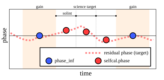
The goal of self-calibration is to determine and correct the residual phase offsets of your science targets from nominal zero after the application of the phase solution from the gain calibrator.

Self-calibration starts with a dataset that would be already science ready. So phase offsets between spectral windows or similar instrumental effects are already gone. If the interpolation of the gain calibrator phases would be perfect, all phases would be zero. However, since that is hardly the case, the goal of self-calibration is to correct the residual phase offsets that are still present, because...

...the atmosphere is changing most likely not changing in the same fashion as the interpolation sheme

...the atmosphere towards your science source can be different from the atmosphere towards your gain calibrator.

With CASA, self-calibration is almost a no-brainer in terms of how to do it (but still you have to make sure that what you do makes sense in an astronomical sense). You have to have a model of your source in the model column of the measurement set. That is typically generated by a first clean of the calibrated data.

Then you iterate through the following steps to get a gradually better and better image quality:

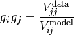
gaincal: Your gain calibration will find the gain correction factors $g_i$ for each antenna for the time interval specified by solint. For antenna-based correction, each baseline has to be corrected by the gain factor $g_ig_j$ that consists of the individual antenna gains $g_i$ and $g_j$ . This factor is given by

$g_i\,g_j = \frac{V^\mathrm{data}_{jj}}{V^\mathrm{model}_{ij}}$

How convenient of CASA that it already wrote the visibility model into the model column! CASA then finds the $N$ gain factors $g_i$ by fitting the visibilities of $N(N-1)/2$ baselines.

applycal: Applying the calibration table to the data will update the corrected column. Then you’re ready for the next iteration.

clean: Cleaning your image will automatically generate a visbility model of the structure that you have just cleaned and write it into the model column.

Examples¶

Continuum self-calibration¶

Dataset: 2011.0.00629.S, two protoplanetary disks (DMTau, MWC480)

Starting Point: calibrated.ms, the result of concatenating the two execution blocks uid___A002_X51d696_X315.ms.split.cal and uid___A002_X51d696_Xef.ms.split.cal.

Spectral Setup: 4 FDM spectral windows with 3840 channels each

Selfcal Target: Continuum of MWC480 (field='4')

Preparing the continuum dataset¶

First we split out the target of interest (MWC480)

os.system('rm -rf MWC480.ms*')
split(vis = 'calibrated.ms',
  outputvis = 'MWC480.ms',
  field = '4',
  datacolumn = 'data')

Then we flag the lines and average the channels to form the continuum dataset MWC480.ms.continuum

flagmanager(vis = 'MWC480.ms',
    mode = 'save',
    versionname = 'Original')

flagdata(vis = 'MWC480.ms',
    mode = 'manual',
    spw = '1:850~1100;2600~2900,2:1800~2200,3:1800~2200',
    flagbackup = F)

split(vis = 'MWC480.ms',
    outputvis = 'MWC480.ms.continuum',
    width = 256,
    timebin = '30s',
    datacolumn = 'data')

flagmanager(vis = 'MWC480.ms',
    mode = 'restore',
    versionname = 'Original')

Starting Self-calibration¶

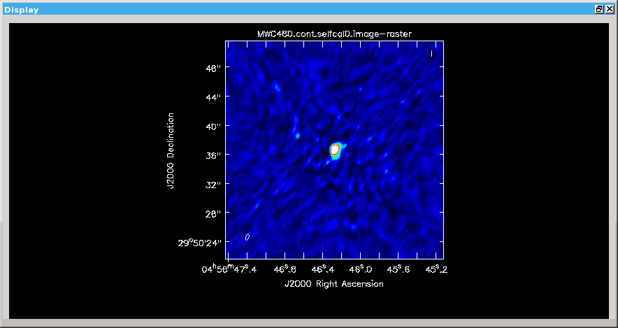
Continuum image of the original data

Self-calibration starts with a first clean, which generates the initial model

os.system('rm -rf MWC480.cont.selfcal*')
clean(vis = 'MWC480.ms.cont',
    imagename = 'MWC480.cont.selfcal0',
    mode = 'mfs',
    outframe = 'LSRK',
    imsize = 300,
    cell = '0.1arcsec',
    mask = 'circle[[147pix,150pix], 23pix]',
    weighting = 'briggs',
    robust = 0.5,
    niter = 1000,
    threshold = '20mJy',
    interactive = F)

The noise level in this image is around 5 mJy/beam. The following iterations will gradually improve the image quality and reduce the noise level.

First Iteration¶

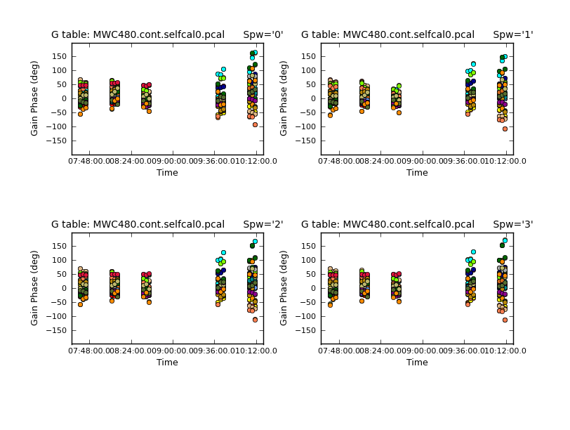
Phase solutions for the first self-calibration step

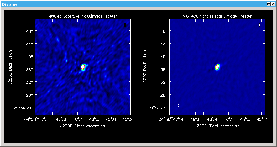
Continuum image of the original data (left) and after the first self-calibration (right). The two colour scales are aligned and highlight the improvement.

As next step follows the gain calibration, which compares the observed visibilities in the data column with the source model in the model column

gaincal(vis = 'MWC480.ms.cont',
    caltable = 'MWC480.cont.selfcal0.pcal',
    calmode = 'p',
    solint = '120s')

In this first iteration we use a solution interval of 2 minutes. Since the gain calibrator is observed every 6 minutes, we get three solutions per scan. These can be displayed with

plotcal(caltable = 'MWC480.cont.selfcal0.pcal',
    xaxis = 'time',
    yaxis = 'phase',
    plotrange = [0,0,-180,180],
    iteration = 'spw',
    subplot = 221,
    figfile = 'MWC480.cont.selfcal0.png')

As you see, the solutions generally group around a phase of zero, but there are some significant correction factors to see - particularly in the last two scans.

The next step is then to apply these solutions to the measurement set

applycal(vis = 'MWC480.ms.cont',
    gaintable = 'MWC480.cont.selfcal0.pcal',
    flagbackup = F)

The corrections are now written into the corrected column, which will in the next iteration be used for the inversion from the Fourier into the image plane.

We will now make a new image, where clean will use the data from the corrected column

os.system('rm -rf MWC480.cont.selfcal1.*')
clean(vis = 'MWC480.ms.cont',
    imagename = 'MWC480.cont.selfcal1',
    field = '0',
    mode = 'mfs',
    outframe = 'LSRK',
    imsize = 300,
    mask = 'MWC480.cont.selfcal0.mask',
    cell = '0.1arcsec',
    weighting = 'briggs',
    robust = 0.5,
    niter = 1000,
    threshold = '5mJy',
    interactive = F)

The improvement in image quality is obvious. The noise level goes down from around 5 mJy/beam to 0.9 mJy/beam.

Second iteration¶

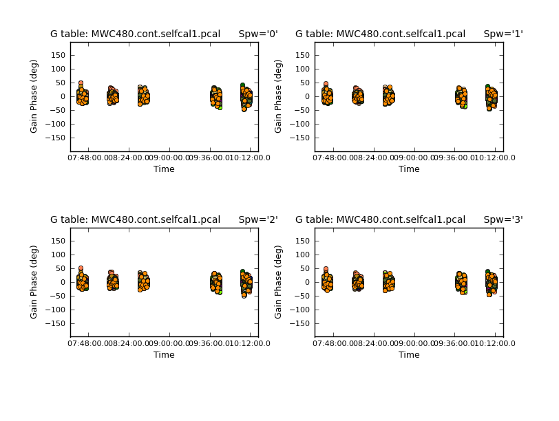
Phase solutions for the first self-calibration step

Continuum image after the first iteration (left) and the second iteration (right). The two colour scales are aligned and highlight the improvement.

Again, we perform a gain calibration to find new correction factors. This time we use a solution interval of the integration time of a single data point solint='int', which in this case is 30 seconds (since we’ve averaged down to 30 seconds when we created this dataset). Moreover, we now apply the first calibration table MWC480.cont.selfcal0.pcal so that the newly created calibration table MWC480.cont.selfcal1.pcal only contains the additional corrections that are needed

gaincal(vis = 'MWC480.ms.cont',
    caltable = 'MWC480.cont.selfcal1.pcal',
    gaintable = ['MWC480.cont.selfcal0.pcal'],
    calmode = 'p',
    solint = 'int')

The results are again displayed

plotcal(caltable = 'MWC480.cont.selfcal1.pcal',
    xaxis = 'time',
    yaxis = 'phase',
    plotrange = [0,0,-180,180],
    iteration = 'spw',
    subplot = 221,
    figfile = 'MWC480.cont.selfcal1.png')

The corrections become less, but still they are up to around 50°.

Again, applying the results to get a new and improved visibilities in the corrected column

applycal(vis = 'MWC480.ms.cont',
    gaintable = ['MWC480.cont.selfcal0.pcal', 'MWC480.cont.selfcal1.pcal'],
    flagbackup = F)

So far, we have only corrected phases. In the next step, we are also correcting for variations in the amplitude gain. Again, we clean the image with the visibilities with the improvements from the last iteration

os.system('rm -rf MWC480.cont.selfcal2.*')
clean(vis = 'MWC480.ms.cont',
    imagename = 'MWC480.cont.selfcal2',
    field = '0',
    mode = 'mfs',
    outframe = 'LSRK',
    imsize = 300,
    mask = 'MWC480.cont.selfcal0.mask',
    cell = '0.1arcsec',
    weighting = 'briggs',
    robust = 0.5,
    niter = 1000,
    threshold = '1mJy',
    interactive = F)

Again, the improvement can be nicely seen. The noise goes down from 0.9 mJy/beam to around 0.5 mJy/beam.

Third Iteration¶

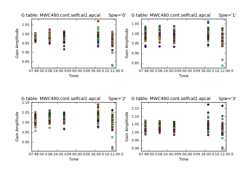
Amplitude correction factors

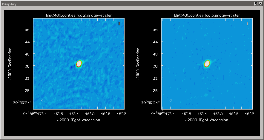
Continuum image after the second iteration (left, phase only) and the iteration (right). The two colour scales are aligned and highlight the improvement.

Now we perform an amplitude gain calibration, where we try to find the average amplitude gain per scan. We do not expect to see any phase variations anymore

gaincal(vis = 'MWC480.ms.cont',
    field = '0',
    caltable = 'MWC480.cont.selfcal2.apcal',
    gaintable = ['MWC480.cont.selfcal0.pcal', 'MWC480.cont.selfcal1.pcal'],
    calmode = 'ap',
    solint = 'inf')

We display the amplitude correction factors (we are not displaying phase correction terms here, as these are indeed zero)

plotcal(caltable = 'MWC480.cont.selfcal2.apcal',
    xaxis = 'time',
    yaxis = 'amp',
    iteration = 'spw',
    subplot = 221,
    figfile = 'MWC480.cont.selfcal2.a.png')

And again applying everything to get the corrected visibilities

applycal(vis = 'MWC480.ms.cont',
    gaintable = ['MWC480.cont.selfcal0.pcal', 'MWC480.cont.selfcal1.pcal', 'MWC480.cont.selfcal2.apcal'],
    flagbackup = F)

Cleaning will show us again the improvement

os.system('rm -rf MWC480.cont.selfcal3*')
clean(vis = 'MWC480.ms.cont',
    imagename = 'MWC480.cont.selfcal3',
    field = '0',
    mode = 'mfs',
    outframe = 'LSRK',
    imsize = 300,
    mask = 'MWC480.cont.selfcal0.mask',
    cell = '0.1arcsec',
    weighting = 'briggs',
    robust = 0.5,
    niter = 1000,
    threshold = '1mJy',
    interactive = F)

And indeed, the noise goes down from 0.5 mJy/beam to around 0.2 mJy/beam.

We started off with a noise level of around 5 mJy/beam and ended up at 0.2 mJy/beam, which is an improvement of around a factor of 25.

Self-Calibration¶

Introduction¶

The Need for Selfcal¶

Selfcal Strategy¶

Examples¶

Continuum self-calibration¶

Preparing the continuum dataset¶

Starting Self-calibration¶

First Iteration¶

Second iteration¶

Third Iteration¶

Table Of Contents

Previous topic

Next topic

This Page

Navigation

Self-Calibration¶

Introduction¶

The Need for Selfcal¶

Selfcal Strategy¶

Examples¶

Continuum self-calibration¶

Preparing the continuum dataset¶

Starting Self-calibration¶

First Iteration¶

Second iteration¶

Third Iteration¶

Table Of Contents

Previous topic

Next topic

This Page

Quick search

Navigation