Making Masks

You may wonder how the 2-dimensional frames in the raw data files are converted to 1-dimensional spectra. Both MIA and EWS use masks for this. Masks contain images with values between 0 and 1 that tell which pixels of the MIDI data should be used (and what weight should be attributed to them - the values in the mask are floating-point numbers). They are stored in files with the same format as MIDI data, so you can use oirGetData and mtv to look at them.

In the past, MIA and EWS used different methods to create the masks. Since MIA+EWS version 1.1, there is one single tool to create, inspect, change, and save the masks. If you are going to use MIA, it will be called automatically, so you don't have to worry too much about the commands explained here, but experts usually want to do everything by themselves, so EWS users might want to read the following carefully.

Create the Mask

To create a mask, we have to find out where the spectrum of the target is in the data frames. To do this, we use the photometric files. Since we later want to check if the mask is at the right position for the interferometric data, we have to specify a fringe search or track file, too. So, the command to create a mask is:

  mask = miamask(files)

where files is an array containing the names of the fringe data, photometry A and photometry B (in that order!). The result mask is an IDL object, but you can ignore that if you are afraid of objects.

The best way to look at the mask is the GUI:

  mask->gui

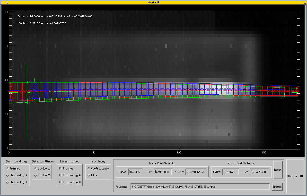
This will open a window like this (click on the image to see larger version):

This GUI allows you to do quite a few things, so the guided tour (no pun intended) will take some time. The larger part is a display of some data, plus an overlay showing the parameters for the mask. At the bottom of the window, there are the controls, which will be explained from left to right in the following.

Background Img

This selects what will be used as background image in the plot: Either the RMS of the fringe data, or the sky-subtracted image of photometry A or B. If you click and drag the left mouse button across the background image, brightness and contrast will change.

Detector Window

Here you select which window you look at. In HIGH_SENS mode, there are two of them for the two outputs of the beamcombiner, while in SCI_PHOT mode, there will be 4 of them, again two for the outputs of the beamcombiner, plus two for the photometry of telescope A and B.

Lines Plotted

This selects which lines are overplotted in the display. This requires some background information:

We started with two photometric files. For both of them, the frames on target and those on the sky are averaged and subtracted from each other. Then, the program searches for the spectrum in each column of the array and fits a 1D Gaussian to it. So, we have a position and width at each column of the image where a spectrum could be found. These are the little green and blue stars and error bars in the plot. Then, a second-order polynomial as function of x is fit to the positions of the Gaussians (called the trace), and a first-order polynomial to their widths. These are indicated by the green and blue lines.

Now, to combine these into one mask, we simply average the results from photometry A and B. This average is shown by the red lines, stars, and error bars. Of course, there are no 1D Gaussians for every column, but the stars and error bars are created from the polynomial fits to make the average better visible.

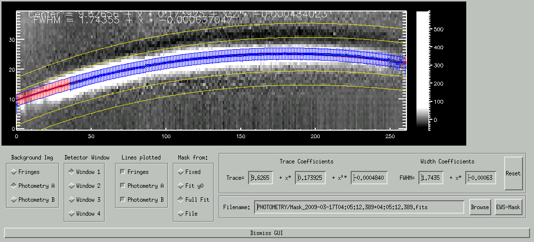
If the selected background image is photometry A or B, and residual background correction via the sky windows is selected (the default), two pairs of yellow lines are plotted outlining the position of the two sky windows, one above the spectrum, and one below. In each column, the background is averaged separately on each side of the spectrum within the sky windows, and a base line is fitted and then subtracted from the spectrum. Here we show examples for both PRISM and GRISM data. Click on the image to see the GRISM plot.

Mask from:

Here you can decide if you like the coefficients obtained by the fits and want to use them to create the mask, or if you'd rather take a mask that you have somewhere in a file. We'll come to the way to select the mask file in a minute. Of course, the mask file has to exist and be readable by you, or the program will refuse to load it. If you use a mask from a file, the colorful lines will vanish (they don't apply any more). Instead, the background image will be mulitplied by the mask to show which part of the image will be used.

Trace coefficients and Width coefficients

These are the coefficients of the first- and second-order fit for the trace and width, resp. More precisely, they are the coefficients obtained by averaging A and B. You can change these coefficients, the new lines will be plotted when you hit return. When you get lost, you can press the Reset-button to the right, to get the results of the fits back. The coefficients entered will actually be used to create the mask (if "Mask from coefficients" is set), so you can use them to specify the mask you think is best for the data.

Filename

This is the name fo the file used for the mask. If "Mask from coefficients" is set, the mask will be written to it (it will overwrite the file without asking!), if "Mask from file" is set, it has to be an existing mask-file. You can enter the filename in the text field, or click on the "Browse"-button to the right to pick a file with the standard IDL file dialog. The default is a name based on date and time of the two photometry files.

This can be used, for example, to select the predefined masks used by EWS. They are stored in the directory "maskfiles" in the MIA+EWS tree and are called

	minrtsMask_FIELD_PRISM_HIGH_SENS_SLIT.fits
	minrtsMask_FIELD_PRISM_SCI_PHOT_SLIT.fits
	minrtsMask_SPECTRAL_GRISM_HIGH_SENS_SLIT.fits
	minrtsMask_SPECTRAL_GRISM_SCI_PHOT_SLIT.fits

Dismiss GUI

If you click here, the GUI will be closed. The settings are stored in the mask-object.

Save the Mask

Now the mask-object knows what kind of mask you want, but it has to be written to a file in order to be used by other programs. This is done with the command:

  mask->write_mask

To make life of programmers easier, this can even be used if the mask is supposed to be loaded from a file. In that case, the mask file will not be overwritten.

Find the Mask

To find out which file actually contains the mask, use

  maskname = mask->get_mask_name()

This is the filename entered in the GUI, i.e. either the file where a newly created mask was stored, or an existing file selected by the user.

Getting rid of the Object

If you created the mask-object with miamask(), then you should destroy it after use in order to recycle the memory:

  obj_destroy, mask

There are more commands associated with a mask-object, they will be described in the reference manual.